

9.6 Topological Optimization with Maximized Stiffness and Heat Transfer
369
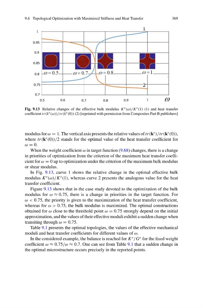
Fig. 9.13 Relative changes of the effective bulk modulus K e (ω)/K e (1) (1) and heat transfer
coefficient tr(k e (ω))/tr(k e (0)) (2) [reprinted with permission from Composites Part B publishers]
modulus for ω = 1. The vertical axis presents the relative values of tr(k
e
)/tr(k
e
(0)),
where tr(k
e
(0))/2 stands for the optimal value of the heat transfer coefficient for
ω = 0.
When the weight coefficient ω in target function (9.68) changes, there is a change
in priorities of optimization from the criterion of the maximum heat transfer coefficient for ω = 0 up to optimization under the criterion of the maximum bulk modulus
or shear modulus.
In Fig. 9.13, curve 1 shows the relative change in the optimal effective bulk
modulus K
e
(ω)/K
e
(1), whereas curve 2 presents the analogous value for the heat
transfer coefficient.
Figure 9.13 shows that in the case study devoted to the optimization of the bulk
modulus for ω ≈ 0.75, there is a change in priorities in the target function. For
ω < 0.75, the priority is given to the maximization of the heat transfer coefficient,
whereas for ω > 0.75, the bulk modulus is maximized. The optimal constructions
obtained for ω close to the threshold point ω = 0.75 strongly depend on the initial
approximation, and the values of their effective moduli exhibit a sudden change when
transiting through ω = 0.75.
Table 9.1 presents the optimal topologies, the values of the effective mechanical
moduli and heat transfer coefficients for different values of ω.
In the considered example, the balance is reached for K
e
/G
e for the fixed weight
coefficient ω ≈ 0.75/ω ≈ 0.7. One can see from Table 9.1 that a sudden change in
the optimal microstructure occurs precisely in the reported points.
369
Fig. 9.13 Relative changes of the effective bulk modulus K e (ω)/K e (1) (1) and heat transfer
coefficient tr(k e (ω))/tr(k e (0)) (2) [reprinted with permission from Composites Part B publishers]
modulus for ω = 1. The vertical axis presents the relative values of tr(k
e
)/tr(k
e
(0)),
where tr(k
e
(0))/2 stands for the optimal value of the heat transfer coefficient for
ω = 0.
When the weight coefficient ω in target function (9.68) changes, there is a change
in priorities of optimization from the criterion of the maximum heat transfer coefficient for ω = 0 up to optimization under the criterion of the maximum bulk modulus
or shear modulus.
In Fig. 9.13, curve 1 shows the relative change in the optimal effective bulk
modulus K
e
(ω)/K
e
(1), whereas curve 2 presents the analogous value for the heat
transfer coefficient.
Figure 9.13 shows that in the case study devoted to the optimization of the bulk
modulus for ω ≈ 0.75, there is a change in priorities in the target function. For
ω < 0.75, the priority is given to the maximization of the heat transfer coefficient,
whereas for ω > 0.75, the bulk modulus is maximized. The optimal constructions
obtained for ω close to the threshold point ω = 0.75 strongly depend on the initial
approximation, and the values of their effective moduli exhibit a sudden change when
transiting through ω = 0.75.
Table 9.1 presents the optimal topologies, the values of the effective mechanical
moduli and heat transfer coefficients for different values of ω.
In the considered example, the balance is reached for K
e
/G
e for the fixed weight
coefficient ω ≈ 0.75/ω ≈ 0.7. One can see from Table 9.1 that a sudden change in
the optimal microstructure occurs precisely in the reported points.