

362
9 Topologic Optimization of Vibrations of Size-Dependent Beams
C
e
i jkl =
1
|Y |
Y
C pqrs
ε
0(i j)
pq − ε
∗(i j)
pq
ε
0(kl)
rs
− ε
∗(kl)
rs
dY,
(9.56)
where ε
∗(i j)
pq =
1
2
∂χ
i j
p
∂ y q
+
∂χ
i j
q
∂ y p
and ε
0(i j)
pq are linearly independent test deformations
on the base cell, employed to define the characteristics of the deformations field
ε
∗(i j)
pq . Here, χ
i j are solutions to the following problem
Y
ε
0(i j)
pq − ε
∗(i j)
pq
C pqrs ε
∗
rs
v
kl
dY ∀v ∈ V Y
defined on the elementary periodic cell, and V Y = v(y) stands for the set of sufficiently smooth functions obtained in Y and exhibiting Y periodicity. For 2D problems,
there are three test deformation fields that take the following form: ε
0(11)
pq
= [1 0 0],
ε
0(22)
pq
= [0 1 0] and ε
0(12)
pq
= [0 0 0.5] [113] (symmetry ε
0(12)
pq
= ε
0(21)
pq implies reduction in the number of test fields from four to three).
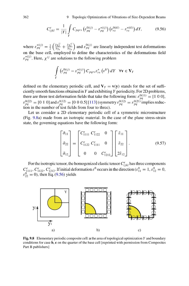
Let us consider a 2D elementary periodic cell of a symmetric microstructure
(Fig. 9.8a) made from an isotropic material. In the case of the plane stress-strain
state, the governing equations have the following form:
⎡
⎢
⎢
⎢
⎢
⎣
¯
σ 11
¯
σ 22
¯
σ 12
⎤
⎥
⎥
⎥
⎥
⎦
=
⎡
⎢
⎢
⎢
⎢
⎣
C
e
1111 C
e
1122
0
C
e
1122 C
e
1111
0
0
0 C
e
1212
⎤
⎥
⎥
⎥
⎥
⎦
⎡
⎢
⎢
⎢
⎢
⎣
¯
ε 11
¯
ε 22
2¯ ε 12
⎤
⎥
⎥
⎥
⎥
⎦
.
(9.57)
For the isotropic tensor, the homogenized elastic tensor C
e
i jkl has three components
C
e
1111 , C
e
1122 , C
e
1212 . If initial deformation ε
0 occurs in the direction (ε
0
11 = 1, ε
0
12 = 0,
ε
0
22 = 0), then Eq. (9.56) yields
Fig. 9.8 Elementary periodic composite cell: a the area of topological optimization Y and boundary
conditions for case b, c on the quarter of the base cell [reprinted with permission from Composites
Part B publishers]
9 Topologic Optimization of Vibrations of Size-Dependent Beams
C
e
i jkl =
1
|Y |
Y
C pqrs
ε
0(i j)
pq − ε
∗(i j)
pq
ε
0(kl)
rs
− ε
∗(kl)
rs
dY,
(9.56)
where ε
∗(i j)
pq =
1
2
∂χ
i j
p
∂ y q
+
∂χ
i j
q
∂ y p
and ε
0(i j)
pq are linearly independent test deformations
on the base cell, employed to define the characteristics of the deformations field
ε
∗(i j)
pq . Here, χ
i j are solutions to the following problem
Y
ε
0(i j)
pq − ε
∗(i j)
pq
C pqrs ε
∗
rs
v
kl
dY ∀v ∈ V Y
defined on the elementary periodic cell, and V Y = v(y) stands for the set of sufficiently smooth functions obtained in Y and exhibiting Y periodicity. For 2D problems,
there are three test deformation fields that take the following form: ε
0(11)
pq
= [1 0 0],
ε
0(22)
pq
= [0 1 0] and ε
0(12)
pq
= [0 0 0.5] [113] (symmetry ε
0(12)
pq
= ε
0(21)
pq implies reduction in the number of test fields from four to three).
Let us consider a 2D elementary periodic cell of a symmetric microstructure
(Fig. 9.8a) made from an isotropic material. In the case of the plane stress-strain
state, the governing equations have the following form:
⎡
⎢
⎢
⎢
⎢
⎣
¯
σ 11
¯
σ 22
¯
σ 12
⎤
⎥
⎥
⎥
⎥
⎦
=
⎡
⎢
⎢
⎢
⎢
⎣
C
e
1111 C
e
1122
0
C
e
1122 C
e
1111
0
0
0 C
e
1212
⎤
⎥
⎥
⎥
⎥
⎦
⎡
⎢
⎢
⎢
⎢
⎣
¯
ε 11
¯
ε 22
2¯ ε 12
⎤
⎥
⎥
⎥
⎥
⎦
.
(9.57)
For the isotropic tensor, the homogenized elastic tensor C
e
i jkl has three components
C
e
1111 , C
e
1122 , C
e
1212 . If initial deformation ε
0 occurs in the direction (ε
0
11 = 1, ε
0
12 = 0,
ε
0
22 = 0), then Eq. (9.56) yields
Fig. 9.8 Elementary periodic composite cell: a the area of topological optimization Y and boundary
conditions for case b, c on the quarter of the base cell [reprinted with permission from Composites
Part B publishers]