

280
7 Mathematical Models of Functionally Graded Beams in Temperature Field
derivatives. Its coefficients allow to carry out a deep analysis regarding the system
behaviour. However, in the current study, our investigations will be limited to only
the main inertial term, assuming that the influence of the remaining inertial terms
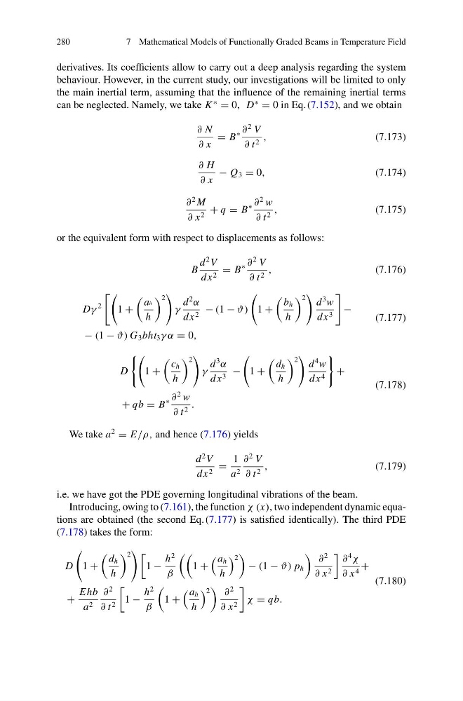
can be neglected. Namely, we take K
∗
= 0, D
∗
= 0 in Eq. (7.152), and we obtain
∂ N
∂ x
= B
∗ ∂
2 V
∂ t 2 ,
(7.173)
∂ H
∂ x
− Q 3 = 0,
(7.174)
∂
2 M
∂ x 2 + q = B
∗ ∂
2 w
∂ t 2 ,
(7.175)
or the equivalent form with respect to displacements as follows:
B
d
2 V
dx 2 = B
∗ ∂
2 V
∂ t 2 ,
(7.176)
Dγ
2
1 +
ah
h
2
γ
d
2
α
dx 2 − (1 − ϑ)
1 +
b h
h
2
d
3 w
dx 3
−
− (1 − ϑ) G 3 bht 3 γ α = 0,
(7.177)
D
1 +
c h
h
2
γ
d
3
α
dx 3 −
1 +
d h
h
2
d
4 w
dx 4
+
+ qb = B
∗ ∂
2 w
∂ t 2 .
(7.178)
We take a
2
= E/ρ, and hence (7.176) yields
d
2 V
dx 2 =
1
a 2
∂
2 V
∂ t 2 ,
(7.179)
i.e. we have got the PDE governing longitudinal vibrations of the beam.
Introducing, owing to (7.161), the function χ (x), two independent dynamic equations are obtained (the second Eq. (7.177) is satisfied identically). The third PDE
(7.178) takes the form:
D
1 +
d h
h
2
1 −
h
2
β
1 +
a h
h
2
− (1 − ϑ) p h
∂
2
∂ x 2
∂
4
χ
∂ x 4 +
+
Ehb
a 2
∂
2
∂ t 2
1 −
h
2
β
1 +
a h
h
2
∂
2
∂ x 2
χ = qb.
(7.180)
7 Mathematical Models of Functionally Graded Beams in Temperature Field
derivatives. Its coefficients allow to carry out a deep analysis regarding the system
behaviour. However, in the current study, our investigations will be limited to only
the main inertial term, assuming that the influence of the remaining inertial terms
can be neglected. Namely, we take K
∗
= 0, D
∗
= 0 in Eq. (7.152), and we obtain
∂ N
∂ x
= B
∗ ∂
2 V
∂ t 2 ,
(7.173)
∂ H
∂ x
− Q 3 = 0,
(7.174)
∂
2 M
∂ x 2 + q = B
∗ ∂
2 w
∂ t 2 ,
(7.175)
or the equivalent form with respect to displacements as follows:
B
d
2 V
dx 2 = B
∗ ∂
2 V
∂ t 2 ,
(7.176)
Dγ
2
1 +
ah
h
2
γ
d
2
α
dx 2 − (1 − ϑ)
1 +
b h
h
2
d
3 w
dx 3
−
− (1 − ϑ) G 3 bht 3 γ α = 0,
(7.177)
D
1 +
c h
h
2
γ
d
3
α
dx 3 −
1 +
d h
h
2
d
4 w
dx 4
+
+ qb = B
∗ ∂
2 w
∂ t 2 .
(7.178)
We take a
2
= E/ρ, and hence (7.176) yields
d
2 V
dx 2 =
1
a 2
∂
2 V
∂ t 2 ,
(7.179)
i.e. we have got the PDE governing longitudinal vibrations of the beam.
Introducing, owing to (7.161), the function χ (x), two independent dynamic equations are obtained (the second Eq. (7.177) is satisfied identically). The third PDE
(7.178) takes the form:
D
1 +
d h
h
2
1 −
h
2
β
1 +
a h
h
2
− (1 − ϑ) p h
∂
2
∂ x 2
∂
4
χ
∂ x 4 +
+
Ehb
a 2
∂
2
∂ t 2
1 −
h
2
β
1 +
a h
h
2
∂
2
∂ x 2
χ = qb.
(7.180)