

7.7 Mathematical Model of Three-Layer Micro- and Nano-Beams
281
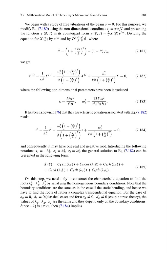
We begin with a study of free vibrations of the beam q ≡ 0. For this purpose, we
modify Eq. (7.180) using the non-dimensional coordinate ξ = π x/L and presenting
the function χ (ξ, t) in its counterpart form χ (ξ, t) =
L
π
X (ξ ) e
iωt . Dividing the
equation for X (ξ ) by e
iωt and by D
h h
2
β
π
6
l 6
˜
ϑ, where
˜
ϑ =
1 +
a h
h
2
− (1 − ϑ) p h ,
(7.181)
we get
X
V I
−
1
k ˜
ϑ
X
I V
−
ω
2
∗
1 +
a h
h
2
˜
ϑ
1 +
d h
h
2 X
I I
+
ω
2
∗
k ˜
ϑ
1 +
d h
h
2 X = 0,
(7.182)
where the following non-dimensional parameters have been introduced
k =
h
2
π
2
l 2 β
,
ω
2
∗ =
12 l
4
ω
2
a 2 h 2 π 4
.
(7.183)
It has been shown in [76] that the characteristic equation associated with Eq. (7.182)
reads:
s
3
−
1
k ˜
ϑ
s
2
−
ω
2
∗
1 +
a h
h
2
˜
ϑ
1 +
dh
h
2
s +
ω
2
∗
k ˜
ϑ
1 +
d h
h
2 = 0,
(7.184)
and consequently, it may have one real and negative root. Introducing the following
notations s 1 = −λ
2
1 , s 2 = λ
2
2 , s 3 = λ
2
3 , the general solution to Eq. (7.182) can be
presented in the following form:
X (ξ ) = C 1 sin(λ 1 ξ) + C 2 cos (λ 1 ξ ) + C 3 sh (λ 2 ξ ) +
+ C 4 ch (λ 1 ξ ) + C 5 sh (λ 3 ξ ) + C 6 ch (λ 3 ξ ) .
(7.185)
On this step, we need only to construct the characteristic equation to find the
roots λ
2
1 , λ
2
2 , λ
2
3 by satisfying the homogeneous boundary conditions. Note that the
boundary conditions are the same as in the case if the static bending, and hence we
have to find the roots of rather a complex transcendental equation. For the case of
a h = 0, d h = 0 (classical case) and for a a h = 0, d h = 0 (couple stress theory), the
values of λ 1 , λ 2 , λ 3 are the same and they depend only on the boundary conditions.
Since −λ
2
1 is a root, then (7.184) implies
281
We begin with a study of free vibrations of the beam q ≡ 0. For this purpose, we
modify Eq. (7.180) using the non-dimensional coordinate ξ = π x/L and presenting
the function χ (ξ, t) in its counterpart form χ (ξ, t) =
L
π
X (ξ ) e
iωt . Dividing the
equation for X (ξ ) by e
iωt and by D
h h
2
β
π
6
l 6
˜
ϑ, where
˜
ϑ =
1 +
a h
h
2
− (1 − ϑ) p h ,
(7.181)
we get
X
V I
−
1
k ˜
ϑ
X
I V
−
ω
2
∗
1 +
a h
h
2
˜
ϑ
1 +
d h
h
2 X
I I
+
ω
2
∗
k ˜
ϑ
1 +
d h
h
2 X = 0,
(7.182)
where the following non-dimensional parameters have been introduced
k =
h
2
π
2
l 2 β
,
ω
2
∗ =
12 l
4
ω
2
a 2 h 2 π 4
.
(7.183)
It has been shown in [76] that the characteristic equation associated with Eq. (7.182)
reads:
s
3
−
1
k ˜
ϑ
s
2
−
ω
2
∗
1 +
a h
h
2
˜
ϑ
1 +
dh
h
2
s +
ω
2
∗
k ˜
ϑ
1 +
d h
h
2 = 0,
(7.184)
and consequently, it may have one real and negative root. Introducing the following
notations s 1 = −λ
2
1 , s 2 = λ
2
2 , s 3 = λ
2
3 , the general solution to Eq. (7.182) can be
presented in the following form:
X (ξ ) = C 1 sin(λ 1 ξ) + C 2 cos (λ 1 ξ ) + C 3 sh (λ 2 ξ ) +
+ C 4 ch (λ 1 ξ ) + C 5 sh (λ 3 ξ ) + C 6 ch (λ 3 ξ ) .
(7.185)
On this step, we need only to construct the characteristic equation to find the
roots λ
2
1 , λ
2
2 , λ
2
3 by satisfying the homogeneous boundary conditions. Note that the
boundary conditions are the same as in the case if the static bending, and hence we
have to find the roots of rather a complex transcendental equation. For the case of
a h = 0, d h = 0 (classical case) and for a a h = 0, d h = 0 (couple stress theory), the
values of λ 1 , λ 2 , λ 3 are the same and they depend only on the boundary conditions.
Since −λ
2
1 is a root, then (7.184) implies