

240
7 Mathematical Models of Functionally Graded Beams in Temperature Field
˜
I = ρ 0 A
h 2
12
1 +
(P E − 1)
2
12
1 +
1
2 (P E − 1)
2
1 +
1
2
P ρ − 1
−
1
6
(P E − 1)
P ρ + 1
1 +
1
2 (P E − 1)
.
Observe that the shear coefficient k s being equal to (5 + 5ν)/(6 + 5ν), is considered to be most suitable for description of the beams with the rectangular cross
section [57].
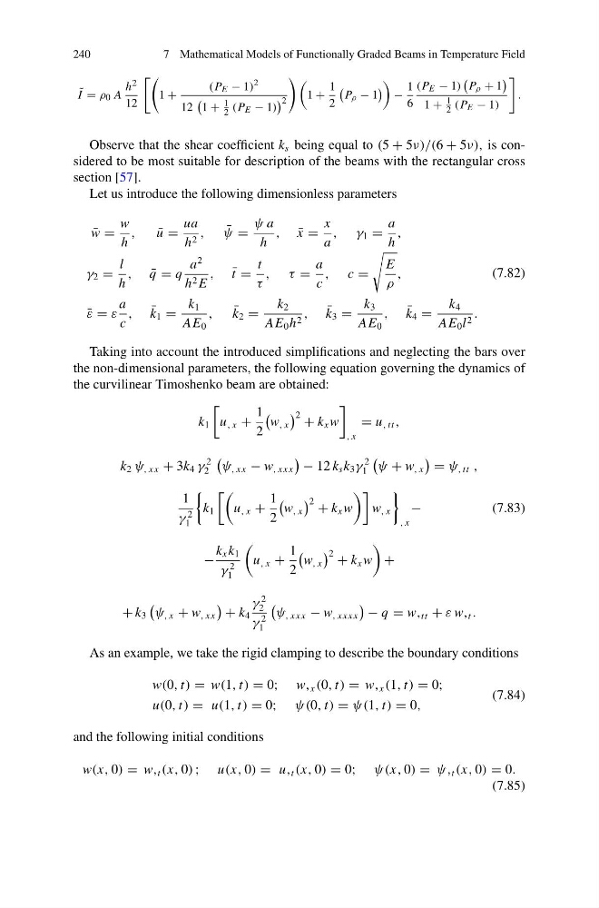
Let us introduce the following dimensionless parameters
¯
w =
w
h
,
¯
u =
ua
h 2 ,
¯
ψ =
ψ a
h
, ¯
x =
x
a
, γ 1 =
a
h
,
γ 2 =
l
h
, ¯
q = q
a
2
h 2 E
, ¯
t =
t
τ
, τ =
a
c
, c =
E
ρ
,
¯
ε = ε
a
c
, ¯
k 1 =
k 1
AE 0
,
¯
k 2 =
k 2
AE 0 h 2 , ¯
k 3 =
k 3
AE 0
, ¯
k 4 =
k 4
AE 0 l 2 .
(7.82)
Taking into account the introduced simplifications and neglecting the bars over
the non-dimensional parameters, the following equation governing the dynamics of
the curvilinear Timoshenko beam are obtained:
k 1
u , x +
1
2
w , x
2 + k x w
, x
= u , tt ,
k 2 ψ , xx + 3k 4 γ
2
2
ψ , xx − w , xxx
− 12 k s k 3 γ
2
1
ψ + w , x
= ψ , tt ,
1
γ
2
1
k 1
u , x +
1
2
w , x
2 + k x w
w , x
, x
−
(7.83)
−
k x k 1
γ
2
1
u , x +
1
2
w , x
2 + k x w
+
+ k 3
ψ , x + w , xx
+ k 4
γ
2
2
γ
2
1
ψ , xxx − w , xxxx
− q = w, tt + ε w, t .
As an example, we take the rigid clamping to describe the boundary conditions
w(0, t) = w(1, t) = 0; w, x (0, t) = w, x (1, t) = 0;
u(0, t) = u(1, t) = 0; ψ(0, t) = ψ(1, t) = 0,
(7.84)
and the following initial conditions
w(x, 0) = w, t (x, 0) ; u(x, 0) = u, t (x, 0) = 0; ψ(x, 0) = ψ, t (x, 0) = 0.
(7.85)
7 Mathematical Models of Functionally Graded Beams in Temperature Field
˜
I = ρ 0 A
h 2
12
1 +
(P E − 1)
2
12
1 +
1
2 (P E − 1)
2
1 +
1
2
P ρ − 1
−
1
6
(P E − 1)
P ρ + 1
1 +
1
2 (P E − 1)
.
Observe that the shear coefficient k s being equal to (5 + 5ν)/(6 + 5ν), is considered to be most suitable for description of the beams with the rectangular cross
section [57].
Let us introduce the following dimensionless parameters
¯
w =
w
h
,
¯
u =
ua
h 2 ,
¯
ψ =
ψ a
h
, ¯
x =
x
a
, γ 1 =
a
h
,
γ 2 =
l
h
, ¯
q = q
a
2
h 2 E
, ¯
t =
t
τ
, τ =
a
c
, c =
E
ρ
,
¯
ε = ε
a
c
, ¯
k 1 =
k 1
AE 0
,
¯
k 2 =
k 2
AE 0 h 2 , ¯
k 3 =
k 3
AE 0
, ¯
k 4 =
k 4
AE 0 l 2 .
(7.82)
Taking into account the introduced simplifications and neglecting the bars over
the non-dimensional parameters, the following equation governing the dynamics of
the curvilinear Timoshenko beam are obtained:
k 1
u , x +
1
2
w , x
2 + k x w
, x
= u , tt ,
k 2 ψ , xx + 3k 4 γ
2
2
ψ , xx − w , xxx
− 12 k s k 3 γ
2
1
ψ + w , x
= ψ , tt ,
1
γ
2
1
k 1
u , x +
1
2
w , x
2 + k x w
w , x
, x
−
(7.83)
−
k x k 1
γ
2
1
u , x +
1
2
w , x
2 + k x w
+
+ k 3
ψ , x + w , xx
+ k 4
γ
2
2
γ
2
1
ψ , xxx − w , xxxx
− q = w, tt + ε w, t .
As an example, we take the rigid clamping to describe the boundary conditions
w(0, t) = w(1, t) = 0; w, x (0, t) = w, x (1, t) = 0;
u(0, t) = u(1, t) = 0; ψ(0, t) = ψ(1, t) = 0,
(7.84)
and the following initial conditions
w(x, 0) = w, t (x, 0) ; u(x, 0) = u, t (x, 0) = 0; ψ(x, 0) = ψ, t (x, 0) = 0.
(7.85)