

7.5 Stability of the Size-Dependent Graded Curvilinear Timoshenko Beams
239
7.5.5 Numerical Results
7.5.5.1 Static Problem of the FGM Size-Dependent Curvilinear
Timoshenko Beam
In order to study the stated problem and to simplify considerations, we assume
G (x, t) = 0, (x, t) = 0, whereas in order to trace the ways of changing the beam
properties with respect to the beam thickness, Young’s modulus E (˜ z), shear modulus
μ (˜ z) and beam thickness ρ (˜ z) are employed.
The properties of the beam material along the beam thickness are defined using
the following linear functions:
E (˜ z) = E 0 +
˜
z +
h
2
h
(E 1 − E 0 ) , μ(˜ z) = μ 0 +
˜
z +
h
2
h
(μ 1 − μ 0 ) ,
ρ (˜ z) = ρ 0 +
˜
z +
h
2
h
(ρ 1 − ρ 0 ) .
(7.78)
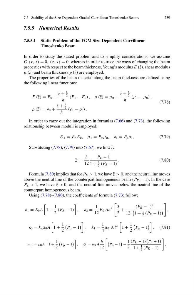
In order to carry out the integration in formulas (7.66) and (7.73), the following
relationship between moduli is employed:
E 1 = P E E 0 , μ 1 = P μ μ 0 , ρ 1 = P ρ ρ 0 ,
(7.79)
Substituting (7.78), (7.79) into (7.67), we find ˜
z:
˜
z =
h
12
P E − 1
1 +
1
2 (P E − 1)
.
(7.80)
Formula (7.80) implies that for P E > 1, we have ˜
z > 0, and the neutral line moves
above the neutral line of the counterpart homogeneous beam (P E = 1). In the case
P E < 1, we have ˜
z < 0, and the neutral line moves below the neutral line of the
counterpart homogeneous beam.
Using (7.78)–(7.80), the coefficients of formula (7.73) follow:
k 1 = E 0 A
1 +
1
2
(P E − 1)
, k 2 =
1
12
E 0 Ah
2
3
2
+
(P E − 1)
2
12
1 +
1
2 (P E − 1)
,
k 3 = k s μ 0 A
1 +
1
2
P μ − 1
, k 4 =
1
4
μ 0 A l
2
1 +
1
2
P μ − 1
, (7.81)
m 0 = ρ 0 A
1 +
1
2
P μ − 1
, Q = ρ 0 A
h
12
P ρ − 1
−
1
2
(P E − 1)
P ρ + 1
1 + 1
2 (P E − 1)
,
239
7.5.5 Numerical Results
7.5.5.1 Static Problem of the FGM Size-Dependent Curvilinear
Timoshenko Beam
In order to study the stated problem and to simplify considerations, we assume
G (x, t) = 0, (x, t) = 0, whereas in order to trace the ways of changing the beam
properties with respect to the beam thickness, Young’s modulus E (˜ z), shear modulus
μ (˜ z) and beam thickness ρ (˜ z) are employed.
The properties of the beam material along the beam thickness are defined using
the following linear functions:
E (˜ z) = E 0 +
˜
z +
h
2
h
(E 1 − E 0 ) , μ(˜ z) = μ 0 +
˜
z +
h
2
h
(μ 1 − μ 0 ) ,
ρ (˜ z) = ρ 0 +
˜
z +
h
2
h
(ρ 1 − ρ 0 ) .
(7.78)
In order to carry out the integration in formulas (7.66) and (7.73), the following
relationship between moduli is employed:
E 1 = P E E 0 , μ 1 = P μ μ 0 , ρ 1 = P ρ ρ 0 ,
(7.79)
Substituting (7.78), (7.79) into (7.67), we find ˜
z:
˜
z =
h
12
P E − 1
1 +
1
2 (P E − 1)
.
(7.80)
Formula (7.80) implies that for P E > 1, we have ˜
z > 0, and the neutral line moves
above the neutral line of the counterpart homogeneous beam (P E = 1). In the case
P E < 1, we have ˜
z < 0, and the neutral line moves below the neutral line of the
counterpart homogeneous beam.
Using (7.78)–(7.80), the coefficients of formula (7.73) follow:
k 1 = E 0 A
1 +
1
2
(P E − 1)
, k 2 =
1
12
E 0 Ah
2
3
2
+
(P E − 1)
2
12
1 +
1
2 (P E − 1)
,
k 3 = k s μ 0 A
1 +
1
2
P μ − 1
, k 4 =
1
4
μ 0 A l
2
1 +
1
2
P μ − 1
, (7.81)
m 0 = ρ 0 A
1 +
1
2
P μ − 1
, Q = ρ 0 A
h
12
P ρ − 1
−
1
2
(P E − 1)
P ρ + 1
1 + 1
2 (P E − 1)
,