

238
7 Mathematical Models of Functionally Graded Beams in Temperature Field
k 2 ψ , x + k 4
ψ , x − w , xx
− ¯
M
x=L
x=0
= 0 or δ ψ|
x=L
x=0 = 0,
k 1
u , x +
1
2
w , x
2 + k x w
w , x + k 3
ψ + w , x
+
+ k 4
ψ , xx − w , xxx
+
C
2
− ¯
V
x=L
x=0
= 0 or δ w|
x=L
x=0 = 0,
k 2 ψ , x + k 4
ψ , x − w , xx
, x
− k 3
ψ + w , x
+
C
2
= Q u , tt + ˜
I ψ , tt , (7.76)
and initial conditions
w(x, 0) = ϕ 1 (x); w (x, 0) , t = ϕ 2 (x);
u(x, 0) = ϕ 3 (x) ; u (x, 0) , t = ϕ 4 (x);
ψ(x, 0) = ϕ 5 (x); ψ (x, 0) , t = ϕ 6 (x),
(7.77)
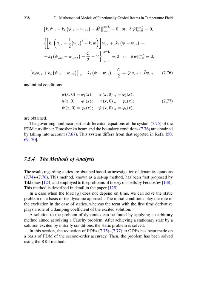
are obtained.
The governing nonlinear partial differential equations of the system (7.75) of the
FGM curvilinear Timoshenko beam and the boundary conditions (7.76) are obtained
by taking into account (7.67). This system differs from that reported in Refs. [50,
69, 70].
7.5.4 The Methods of Analysis
The results regarding statics are obtained based on investigation of dynamic equations
(7.74)–(7.76). This method, known as a set-up method, has been first proposed by
Tikhonov [124] and employed to the problems of theory of shells by Feodos’ev [138].
This method is described in detail in the paper [125].
In a case when the load [ ¯
q] does not depend on time, we can solve the static
problem on a basis of the dynamic approach. The initial conditions play the role of
the excitation in the case of statics, whereas the term with the first time derivative
plays a role of a damping coefficient of the excited solution.
A solution to the problem of dynamics can be found by applying an arbitrary
method aimed at solving a Cauchy problem. After achieving a stationary state by a
solution excited by initially conditions, the static problem is solved.
In this section, the reduction of PDEs (7.75)–(7.77) to ODEs has been made on
a basis of FDM of the second-order accuracy. Then, the problem has been solved
using the RK4 method.
7 Mathematical Models of Functionally Graded Beams in Temperature Field
k 2 ψ , x + k 4
ψ , x − w , xx
− ¯
M
x=L
x=0
= 0 or δ ψ|
x=L
x=0 = 0,
k 1
u , x +
1
2
w , x
2 + k x w
w , x + k 3
ψ + w , x
+
+ k 4
ψ , xx − w , xxx
+
C
2
− ¯
V
x=L
x=0
= 0 or δ w|
x=L
x=0 = 0,
k 2 ψ , x + k 4
ψ , x − w , xx
, x
− k 3
ψ + w , x
+
C
2
= Q u , tt + ˜
I ψ , tt , (7.76)
and initial conditions
w(x, 0) = ϕ 1 (x); w (x, 0) , t = ϕ 2 (x);
u(x, 0) = ϕ 3 (x) ; u (x, 0) , t = ϕ 4 (x);
ψ(x, 0) = ϕ 5 (x); ψ (x, 0) , t = ϕ 6 (x),
(7.77)
are obtained.
The governing nonlinear partial differential equations of the system (7.75) of the
FGM curvilinear Timoshenko beam and the boundary conditions (7.76) are obtained
by taking into account (7.67). This system differs from that reported in Refs. [50,
69, 70].
7.5.4 The Methods of Analysis
The results regarding statics are obtained based on investigation of dynamic equations
(7.74)–(7.76). This method, known as a set-up method, has been first proposed by
Tikhonov [124] and employed to the problems of theory of shells by Feodos’ev [138].
This method is described in detail in the paper [125].
In a case when the load [ ¯
q] does not depend on time, we can solve the static
problem on a basis of the dynamic approach. The initial conditions play the role of
the excitation in the case of statics, whereas the term with the first time derivative
plays a role of a damping coefficient of the excited solution.
A solution to the problem of dynamics can be found by applying an arbitrary
method aimed at solving a Cauchy problem. After achieving a stationary state by a
solution excited by initially conditions, the static problem is solved.
In this section, the reduction of PDEs (7.75)–(7.77) to ODEs has been made on
a basis of FDM of the second-order accuracy. Then, the problem has been solved
using the RK4 method.