

7.4 Chaotic Dynamics of Size-Dependent Graded Timoshenko Beams
219
k 1
u , x +
1
2
w , x
2
, x
= u , tt ,
k 2 ψ , xx + 3k 4 γ
2
2
ψ , xx − w , xxx
− 12 k s k 3 γ
2
1
ψ + w , x
= ψ , tt ,
(7.51)
1
γ
2
1
k 1
u , x +
1
2
w , x
2
w , x
, x
+ k 3
ψ , x + w , xx
+
+ k 4
γ
2
2
γ
2
1
ψ , xxx − w , xxxx
+ q = w, tt + ε w, t
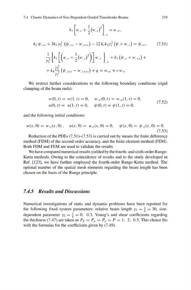
We restrict further considerations to the following boundary conditions (rigid
clamping of the beam ends):
w(0, t) = w(1, t) = 0, w, x (0, t) = w, x (1, t) = 0,
u(0, t) = u(1, t) = 0, ψ(0, t) = ψ(1, t) = 0,
(7.52)
and the following initial conditions:
w(x, 0) = w, t (x, 0) , u(x, 0) = u, t (x, 0) = 0, ψ(x, 0) = ψ, t (x, 0) = 0.
(7.53)
Reduction of the PDEs (7.51)–(7.53) is carried out by means the finite difference
method (FDM) of the second-order accuracy, and the finite element method (FEM).
Both FDM and FEM are used to validate the results.
We have compared numerical results yielded by the fourth- and sixth-order RungeKutta methods. Owing to the coincidence of results and to the study developed in
Ref. [123], we have further employed the fourth-order Runge-Kutta method. The
optimal number of the spatial mesh elements regarding the beam length has been
chosen on the basis of the Runge principle.
7.4.5 Results and Discussions
Numerical investigations of static and dynamic problems have been reported for
the following fixed system parameters: relative beam length γ 1 =
a
h
= 30, sizedependent parameter γ 2 =
l
h
= 0; 0.3. Young’s and shear coefficients regarding
the thickness (7.47) are taken as P E = P μ = P ρ = P = 1; 2; 0.5. This choice fits
with the formulas for the coefficients given by (7.49).
219
k 1
u , x +
1
2
w , x
2
, x
= u , tt ,
k 2 ψ , xx + 3k 4 γ
2
2
ψ , xx − w , xxx
− 12 k s k 3 γ
2
1
ψ + w , x
= ψ , tt ,
(7.51)
1
γ
2
1
k 1
u , x +
1
2
w , x
2
w , x
, x
+ k 3
ψ , x + w , xx
+
+ k 4
γ
2
2
γ
2
1
ψ , xxx − w , xxxx
+ q = w, tt + ε w, t
We restrict further considerations to the following boundary conditions (rigid
clamping of the beam ends):
w(0, t) = w(1, t) = 0, w, x (0, t) = w, x (1, t) = 0,
u(0, t) = u(1, t) = 0, ψ(0, t) = ψ(1, t) = 0,
(7.52)
and the following initial conditions:
w(x, 0) = w, t (x, 0) , u(x, 0) = u, t (x, 0) = 0, ψ(x, 0) = ψ, t (x, 0) = 0.
(7.53)
Reduction of the PDEs (7.51)–(7.53) is carried out by means the finite difference
method (FDM) of the second-order accuracy, and the finite element method (FEM).
Both FDM and FEM are used to validate the results.
We have compared numerical results yielded by the fourth- and sixth-order RungeKutta methods. Owing to the coincidence of results and to the study developed in
Ref. [123], we have further employed the fourth-order Runge-Kutta method. The
optimal number of the spatial mesh elements regarding the beam length has been
chosen on the basis of the Runge principle.
7.4.5 Results and Discussions
Numerical investigations of static and dynamic problems have been reported for
the following fixed system parameters: relative beam length γ 1 =
a
h
= 30, sizedependent parameter γ 2 =
l
h
= 0; 0.3. Young’s and shear coefficients regarding
the thickness (7.47) are taken as P E = P μ = P ρ = P = 1; 2; 0.5. This choice fits
with the formulas for the coefficients given by (7.49).