

218
7 Mathematical Models of Functionally Graded Beams in Temperature Field
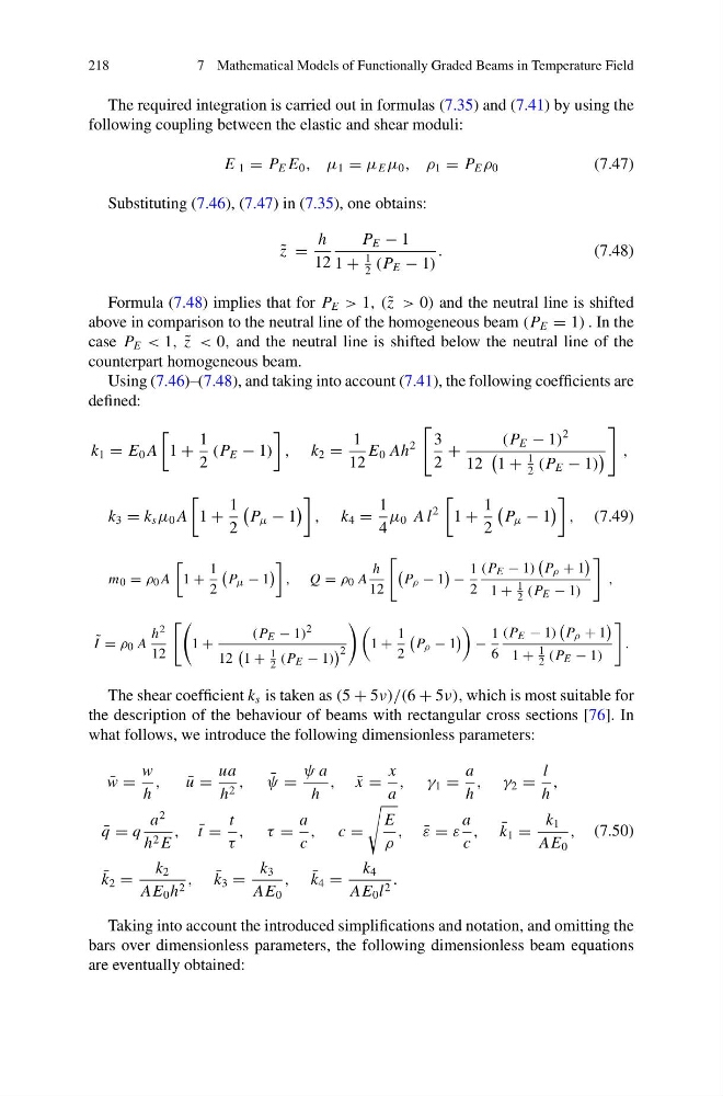
The required integration is carried out in formulas (7.35) and (7.41) by using the
following coupling between the elastic and shear moduli:
E 1 = P E E 0 , μ 1 = μ E μ 0 , ρ 1 = P E ρ 0
(7.47)
Substituting (7.46), (7.47) in (7.35), one obtains:
˜
z =
h
12
P E − 1
1 +
1
2 (P E − 1)
.
(7.48)
Formula (7.48) implies that for P E > 1, (˜ z > 0) and the neutral line is shifted
above in comparison to the neutral line of the homogeneous beam (P E = 1) . In the
case P E < 1, ˜
z < 0, and the neutral line is shifted below the neutral line of the
counterpart homogeneous beam.
Using (7.46)–(7.48), and taking into account (7.41), the following coefficients are
defined:
k 1 = E 0 A
1 +
1
2
(P E − 1)
, k 2 =
1
12
E 0 Ah
2
3
2
+
(P E − 1)
2
12
1 +
1
2 (P E − 1)
,
k 3 = k s μ 0 A
1 +
1
2
P μ − 1
, k 4 =
1
4
μ 0 A l
2
1 +
1
2
P μ − 1
, (7.49)
m 0 = ρ 0 A
1 +
1
2
P μ − 1
, Q = ρ 0 A
h
12
P ρ − 1
−
1
2
(P E − 1)
P ρ + 1
1 +
1
2 (P E − 1)
,
˜
I = ρ 0 A
h 2
12
1 +
(P E − 1)
2
12
1 +
1
2 (P E − 1)
2
1 +
1
2
P ρ − 1
−
1
6
(P E − 1)
P ρ + 1
1 +
1
2 (P E − 1)
.
The shear coefficient k s is taken as (5 + 5ν)/(6 + 5ν), which is most suitable for
the description of the behaviour of beams with rectangular cross sections [76]. In
what follows, we introduce the following dimensionless parameters:
¯
w =
w
h
,
¯
u =
ua
h 2 ,
¯
ψ =
ψ a
h
, ¯
x =
x
a
, γ 1 =
a
h
, γ 2 =
l
h
,
¯
q = q
a
2
h 2 E
, ¯
t =
t
τ
, τ =
a
c
, c =
E
ρ
, ¯
ε = ε
a
c
, ¯
k 1 =
k 1
AE 0
,
¯
k 2 =
k 2
AE 0 h 2 , ¯
k 3 =
k 3
AE 0
, ¯
k 4 =
k 4
AE 0 l 2 .
(7.50)
Taking into account the introduced simplifications and notation, and omitting the
bars over dimensionless parameters, the following dimensionless beam equations
are eventually obtained:
7 Mathematical Models of Functionally Graded Beams in Temperature Field
The required integration is carried out in formulas (7.35) and (7.41) by using the
following coupling between the elastic and shear moduli:
E 1 = P E E 0 , μ 1 = μ E μ 0 , ρ 1 = P E ρ 0
(7.47)
Substituting (7.46), (7.47) in (7.35), one obtains:
˜
z =
h
12
P E − 1
1 +
1
2 (P E − 1)
.
(7.48)
Formula (7.48) implies that for P E > 1, (˜ z > 0) and the neutral line is shifted
above in comparison to the neutral line of the homogeneous beam (P E = 1) . In the
case P E < 1, ˜
z < 0, and the neutral line is shifted below the neutral line of the
counterpart homogeneous beam.
Using (7.46)–(7.48), and taking into account (7.41), the following coefficients are
defined:
k 1 = E 0 A
1 +
1
2
(P E − 1)
, k 2 =
1
12
E 0 Ah
2
3
2
+
(P E − 1)
2
12
1 +
1
2 (P E − 1)
,
k 3 = k s μ 0 A
1 +
1
2
P μ − 1
, k 4 =
1
4
μ 0 A l
2
1 +
1
2
P μ − 1
, (7.49)
m 0 = ρ 0 A
1 +
1
2
P μ − 1
, Q = ρ 0 A
h
12
P ρ − 1
−
1
2
(P E − 1)
P ρ + 1
1 +
1
2 (P E − 1)
,
˜
I = ρ 0 A
h 2
12
1 +
(P E − 1)
2
12
1 +
1
2 (P E − 1)
2
1 +
1
2
P ρ − 1
−
1
6
(P E − 1)
P ρ + 1
1 +
1
2 (P E − 1)
.
The shear coefficient k s is taken as (5 + 5ν)/(6 + 5ν), which is most suitable for
the description of the behaviour of beams with rectangular cross sections [76]. In
what follows, we introduce the following dimensionless parameters:
¯
w =
w
h
,
¯
u =
ua
h 2 ,
¯
ψ =
ψ a
h
, ¯
x =
x
a
, γ 1 =
a
h
, γ 2 =
l
h
,
¯
q = q
a
2
h 2 E
, ¯
t =
t
τ
, τ =
a
c
, c =
E
ρ
, ¯
ε = ε
a
c
, ¯
k 1 =
k 1
AE 0
,
¯
k 2 =
k 2
AE 0 h 2 , ¯
k 3 =
k 3
AE 0
, ¯
k 4 =
k 4
AE 0 l 2 .
(7.50)
Taking into account the introduced simplifications and notation, and omitting the
bars over dimensionless parameters, the following dimensionless beam equations
are eventually obtained: