

7.4 Chaotic Dynamics of Size-Dependent Graded Timoshenko Beams
217
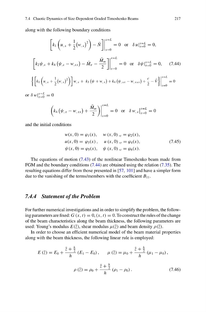
along with the following boundary conditions
k 1
u , x +
1
2
w , x
2
− ¯
N
x=L
x=0
= 0 or δ u|
x=L
x=0 = 0,
k 2 ψ ,x + k 4
ψ ,x − w ,xx
− ¯
M σ −
¯
M m
2
x=L
x=0
= 0 or δψ|
x=L
x=0 = 0,
(7.44)
k 1
u , x +
1
2
w , x
2
w , x + k 3
ψ + w , x
+ k 4
ψ , xx − w , xxx
+
c
2
− ¯
V
x=L
x=0
= 0
or δ w|
x=L
x=0 = 0
k 4
ψ , x − w , xx
+
¯
M m
2
x=L
x=0
= 0 or δ w , x
x=L
x=0
= 0
and the initial conditions
w(x, 0) = ϕ 1 (x), w (x, 0) , t = ϕ 2 (x),
u(x, 0) = ϕ 3 (x) , u (x, 0) , t = ϕ 4 (x),
ψ(x, 0) = ϕ 5 (x), ψ (x, 0) , t = ϕ 6 (x).
(7.45)
The equations of motion (7.43) of the nonlinear Timoshenko beam made from
FGM and the boundary conditions (7.44) are obtained using the relation (7.35). The
resulting equations differ from those presented in [57, 101] and have a simpler form
due to the vanishing of the terms/members with the coefficient B 11 .
7.4.4 Statement of the Problem
For further numerical investigations and in order to simplify the problem, the following parameters are fixed: G (x, t) = 0, (x, t) = 0. To construct the rules of the change
of the beam characteristics along the beam thickness, the following parameters are
used: Young’s modulus E(˜ z), shear modulus μ(˜ z) and beam density ρ(˜ z).
In order to choose an efficient numerical model of the beam material properties
along with the beam thickness, the following linear rule is employed:
E (˜ z) = E 0 +
˜
z +
h
2
h
(E 1 − E 0 ) ,
μ(˜ z) = μ 0 +
˜
z +
h
2
h
(μ 1 − μ 0 ) ,
ρ (˜ z) = ρ 0 +
˜
z +
h
2
h
(ρ 1 − ρ 0 ) .
(7.46)
217
along with the following boundary conditions
k 1
u , x +
1
2
w , x
2
− ¯
N
x=L
x=0
= 0 or δ u|
x=L
x=0 = 0,
k 2 ψ ,x + k 4
ψ ,x − w ,xx
− ¯
M σ −
¯
M m
2
x=L
x=0
= 0 or δψ|
x=L
x=0 = 0,
(7.44)
k 1
u , x +
1
2
w , x
2
w , x + k 3
ψ + w , x
+ k 4
ψ , xx − w , xxx
+
c
2
− ¯
V
x=L
x=0
= 0
or δ w|
x=L
x=0 = 0
k 4
ψ , x − w , xx
+
¯
M m
2
x=L
x=0
= 0 or δ w , x
x=L
x=0
= 0
and the initial conditions
w(x, 0) = ϕ 1 (x), w (x, 0) , t = ϕ 2 (x),
u(x, 0) = ϕ 3 (x) , u (x, 0) , t = ϕ 4 (x),
ψ(x, 0) = ϕ 5 (x), ψ (x, 0) , t = ϕ 6 (x).
(7.45)
The equations of motion (7.43) of the nonlinear Timoshenko beam made from
FGM and the boundary conditions (7.44) are obtained using the relation (7.35). The
resulting equations differ from those presented in [57, 101] and have a simpler form
due to the vanishing of the terms/members with the coefficient B 11 .
7.4.4 Statement of the Problem
For further numerical investigations and in order to simplify the problem, the following parameters are fixed: G (x, t) = 0, (x, t) = 0. To construct the rules of the change
of the beam characteristics along the beam thickness, the following parameters are
used: Young’s modulus E(˜ z), shear modulus μ(˜ z) and beam density ρ(˜ z).
In order to choose an efficient numerical model of the beam material properties
along with the beam thickness, the following linear rule is employed:
E (˜ z) = E 0 +
˜
z +
h
2
h
(E 1 − E 0 ) ,
μ(˜ z) = μ 0 +
˜
z +
h
2
h
(μ 1 − μ 0 ) ,
ρ (˜ z) = ρ 0 +
˜
z +
h
2
h
(ρ 1 − ρ 0 ) .
(7.46)