

166
6 Mathematical Models of Micro- and Nano-cylindrical Panels in Temperature Field
w(x, 0) =
∂w (x, t)
∂t
t=0
= 0,
u(x, 0) =
∂u (x, t)
∂t
t=0
= 0.
(6.133)
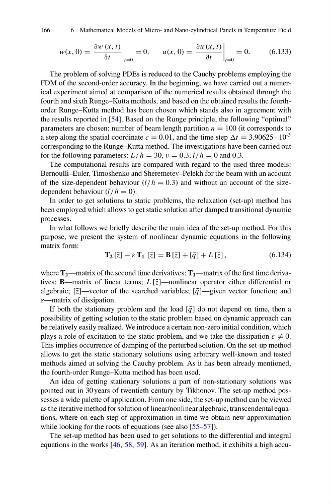
The problem of solving PDEs is reduced to the Cauchy problems employing the
FDM of the second-order accuracy. In the beginning, we have carried out a numerical experiment aimed at comparison of the numerical results obtained through the
fourth and sixth Runge–Kutta methods, and based on the obtained results the fourthorder Runge–Kutta method has been chosen which stands also in agreement with
the results reported in [54]. Based on the Runge principle, the following “optimal”
parameters are chosen: number of beam length partition n = 100 (it corresponds to
a step along the spatial coordinate c = 0.01, and the time step t = 3.90625 · 10
-3
corresponding to the Runge–Kutta method. The investigations have been carried out
for the following parameters: L/ h = 30, ν = 0.3, l/ h = 0 and 0.3.
The computational results are compared with regard to the used three models:
Bernoulli–Euler, Timoshenko and Sheremetev–Pelekh for the beam with an account
of the size-dependent behaviour (l/ h = 0.3) and without an account of the sizedependent behaviour (l/ h = 0).
In order to get solutions to static problems, the relaxation (set-up) method has
been employed which allows to get static solution after damped transitional dynamic
processes.
In what follows we briefly describe the main idea of the set-up method. For this
purpose, we present the system of nonlinear dynamic equations in the following
matrix form:
T 2 [¯ z] + ε T 1 [¯ z] = B [¯ z] + [ ¯
q] + L [¯ z] ,
(6.134)
where T 2 —matrix of the second time derivatives; T 1 —matrix of the first time derivatives; B—matrix of linear terms; L [¯ z]—nonlinear operator either differential or
algebraic; [¯ z]—vector of the searched variables; [ ¯
q]—given vector function; and
ε—matrix of dissipation.
If both the stationary problem and the load [ ¯
q] do not depend on time, then a
possibility of getting solution to the static problem based on dynamic approach can
be relatively easily realized. We introduce a certain non-zero initial condition, which
plays a role of excitation to the static problem, and we take the dissipation ε = 0.
This implies occurrence of damping of the perturbed solution. On the set-up method
allows to get the static stationary solutions using arbitrary well-known and tested
methods aimed at solving the Cauchy problem. As it has been already mentioned,
the fourth-order Runge–Kutta method has been used.
An idea of getting stationary solutions a part of non-stationary solutions was
pointed out in 30 years of twentieth century by Tikhonov. The set-up method possesses a wide palette of application. From one side, the set-up method can be viewed
as the iterative method for solution of linear/nonlinear algebraic, transcendental equations, where on each step of approximation in time we obtain new approximation
while looking for the roots of equations (see also [55–57]).
The set-up method has been used to get solutions to the differential and integral
equations in the works [46, 58, 59]. As an iteration method, it exhibits a high accu-
6 Mathematical Models of Micro- and Nano-cylindrical Panels in Temperature Field
w(x, 0) =
∂w (x, t)
∂t
t=0
= 0,
u(x, 0) =
∂u (x, t)
∂t
t=0
= 0.
(6.133)
The problem of solving PDEs is reduced to the Cauchy problems employing the
FDM of the second-order accuracy. In the beginning, we have carried out a numerical experiment aimed at comparison of the numerical results obtained through the
fourth and sixth Runge–Kutta methods, and based on the obtained results the fourthorder Runge–Kutta method has been chosen which stands also in agreement with
the results reported in [54]. Based on the Runge principle, the following “optimal”
parameters are chosen: number of beam length partition n = 100 (it corresponds to
a step along the spatial coordinate c = 0.01, and the time step t = 3.90625 · 10
-3
corresponding to the Runge–Kutta method. The investigations have been carried out
for the following parameters: L/ h = 30, ν = 0.3, l/ h = 0 and 0.3.
The computational results are compared with regard to the used three models:
Bernoulli–Euler, Timoshenko and Sheremetev–Pelekh for the beam with an account
of the size-dependent behaviour (l/ h = 0.3) and without an account of the sizedependent behaviour (l/ h = 0).
In order to get solutions to static problems, the relaxation (set-up) method has
been employed which allows to get static solution after damped transitional dynamic
processes.
In what follows we briefly describe the main idea of the set-up method. For this
purpose, we present the system of nonlinear dynamic equations in the following
matrix form:
T 2 [¯ z] + ε T 1 [¯ z] = B [¯ z] + [ ¯
q] + L [¯ z] ,
(6.134)
where T 2 —matrix of the second time derivatives; T 1 —matrix of the first time derivatives; B—matrix of linear terms; L [¯ z]—nonlinear operator either differential or
algebraic; [¯ z]—vector of the searched variables; [ ¯
q]—given vector function; and
ε—matrix of dissipation.
If both the stationary problem and the load [ ¯
q] do not depend on time, then a
possibility of getting solution to the static problem based on dynamic approach can
be relatively easily realized. We introduce a certain non-zero initial condition, which
plays a role of excitation to the static problem, and we take the dissipation ε = 0.
This implies occurrence of damping of the perturbed solution. On the set-up method
allows to get the static stationary solutions using arbitrary well-known and tested
methods aimed at solving the Cauchy problem. As it has been already mentioned,
the fourth-order Runge–Kutta method has been used.
An idea of getting stationary solutions a part of non-stationary solutions was
pointed out in 30 years of twentieth century by Tikhonov. The set-up method possesses a wide palette of application. From one side, the set-up method can be viewed
as the iterative method for solution of linear/nonlinear algebraic, transcendental equations, where on each step of approximation in time we obtain new approximation
while looking for the roots of equations (see also [55–57]).
The set-up method has been used to get solutions to the differential and integral
equations in the works [46, 58, 59]. As an iteration method, it exhibits a high accu-