

6.5 Static Solutions
167
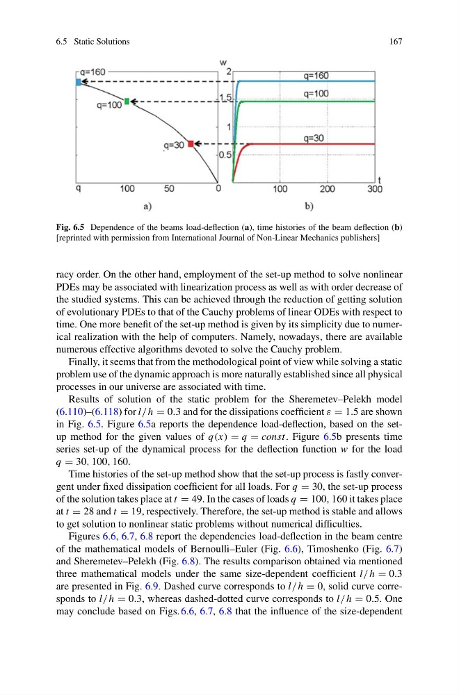
Fig. 6.5 Dependence of the beams load-deflection (a), time histories of the beam deflection (b)
[reprinted with permission from International Journal of Non-Linear Mechanics publishers]
racy order. On the other hand, employment of the set-up method to solve nonlinear
PDEs may be associated with linearization process as well as with order decrease of
the studied systems. This can be achieved through the reduction of getting solution
of evolutionary PDEs to that of the Cauchy problems of linear ODEs with respect to
time. One more benefit of the set-up method is given by its simplicity due to numerical realization with the help of computers. Namely, nowadays, there are available
numerous effective algorithms devoted to solve the Cauchy problem.
Finally, it seems that from the methodological point of view while solving a static
problem use of the dynamic approach is more naturally established since all physical
processes in our universe are associated with time.
Results of solution of the static problem for the Sheremetev–Pelekh model
(6.110)–(6.118) for l/ h = 0.3 and for the dissipations coefficient ε = 1.5 are shown
in Fig. 6.5. Figure 6.5a reports the dependence load-deflection, based on the setup method for the given values of q(x) = q = const. Figure 6.5b presents time
series set-up of the dynamical process for the deflection function w for the load
q = 30, 100, 160.
Time histories of the set-up method show that the set-up process is fastly convergent under fixed dissipation coefficient for all loads. For q = 30, the set-up process
of the solution takes place at t = 49. In the cases of loads q = 100, 160 it takes place
at t = 28 and t = 19, respectively. Therefore, the set-up method is stable and allows
to get solution to nonlinear static problems without numerical difficulties.
Figures 6.6, 6.7, 6.8 report the dependencies load-deflection in the beam centre
of the mathematical models of Bernoulli–Euler (Fig. 6.6), Timoshenko (Fig. 6.7)
and Sheremetev–Pelekh (Fig. 6.8). The results comparison obtained via mentioned
three mathematical models under the same size-dependent coefficient l/ h = 0.3
are presented in Fig. 6.9. Dashed curve corresponds to l/ h = 0, solid curve corresponds to l/ h = 0.3, whereas dashed-dotted curve corresponds to l/ h = 0.5. One
may conclude based on Figs. 6.6, 6.7, 6.8 that the influence of the size-dependent
167
Fig. 6.5 Dependence of the beams load-deflection (a), time histories of the beam deflection (b)
[reprinted with permission from International Journal of Non-Linear Mechanics publishers]
racy order. On the other hand, employment of the set-up method to solve nonlinear
PDEs may be associated with linearization process as well as with order decrease of
the studied systems. This can be achieved through the reduction of getting solution
of evolutionary PDEs to that of the Cauchy problems of linear ODEs with respect to
time. One more benefit of the set-up method is given by its simplicity due to numerical realization with the help of computers. Namely, nowadays, there are available
numerous effective algorithms devoted to solve the Cauchy problem.
Finally, it seems that from the methodological point of view while solving a static
problem use of the dynamic approach is more naturally established since all physical
processes in our universe are associated with time.
Results of solution of the static problem for the Sheremetev–Pelekh model
(6.110)–(6.118) for l/ h = 0.3 and for the dissipations coefficient ε = 1.5 are shown
in Fig. 6.5. Figure 6.5a reports the dependence load-deflection, based on the setup method for the given values of q(x) = q = const. Figure 6.5b presents time
series set-up of the dynamical process for the deflection function w for the load
q = 30, 100, 160.
Time histories of the set-up method show that the set-up process is fastly convergent under fixed dissipation coefficient for all loads. For q = 30, the set-up process
of the solution takes place at t = 49. In the cases of loads q = 100, 160 it takes place
at t = 28 and t = 19, respectively. Therefore, the set-up method is stable and allows
to get solution to nonlinear static problems without numerical difficulties.
Figures 6.6, 6.7, 6.8 report the dependencies load-deflection in the beam centre
of the mathematical models of Bernoulli–Euler (Fig. 6.6), Timoshenko (Fig. 6.7)
and Sheremetev–Pelekh (Fig. 6.8). The results comparison obtained via mentioned
three mathematical models under the same size-dependent coefficient l/ h = 0.3
are presented in Fig. 6.9. Dashed curve corresponds to l/ h = 0, solid curve corresponds to l/ h = 0.3, whereas dashed-dotted curve corresponds to l/ h = 0.5. One
may conclude based on Figs. 6.6, 6.7, 6.8 that the influence of the size-dependent