

6.5 Static Solutions
165
w|
x=1
x=0 = 0,
∂ϕ
∂ x
−
∂
2 w
∂ x 2
x=1
x=0
= 0
or
∂w
∂ x
x=1
x=0
= 0.
(6.126)
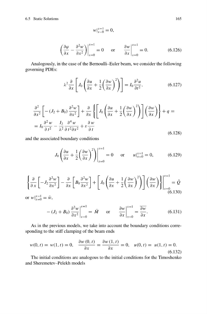
Analogously, in the case of the Bernoulli–Euler beam, we consider the following
governing PDEs:
λ
2 ∂
∂ x
J 0
∂u
∂ x
+
1
2
∂w
∂ x
2
= I 0
∂
2 u
∂t 2 ,
(6.127)
∂
2
∂ x 2
− (J 2 + B 0 )
∂
2 w
∂ x 2
+
∂
∂ x
J 0
∂u
∂ x
+
1
2
∂w
∂ x
2
∂w
∂ x
+ q =
= I 0
∂
2 w
∂ t 2 −
I 2
λ 2
∂
4 w
∂ t 2 ∂ x 2 + ε
∂ w
∂ t
(6.128)
and the associated boundary conditions
J 0
∂u
∂ x
+
1
2
∂w
∂ x
2
x=1
x=0
= 0
or
u|
x=1
x=0 = 0,
(6.129)
∂
∂ x
−J 2
∂
2 w
∂ x 2
−
∂
∂ x
B 0
∂
2 w
∂ x 2
+
J 0
∂u
∂ x
+
1
2
∂w
∂ x
2
∂w
∂ x
x=1
x=0
= ¯
Q
(6.130)
or w|
x=1
x=0 = ¯
w,
− (J 2 + B 0 )
∂
2 w
∂ x 2
x=1
x=0
= ¯
M
or
∂w
∂ x
x=1
x=0
=
____
∂w
∂ x
.
(6.131)
As in the previous models, we take into account the boundary conditions corresponding to the stiff clamping of the beam ends
w(0, t) = w(1, t) = 0,
∂w (0, t)
∂ x
=
∂w (1, t)
∂ x
= 0, u(0, t) = u(1, t) = 0.
(6.132)
The initial conditions are analogous to the initial conditions for the Timoshenko
and Sheremetev–Pelekh models
165
w|
x=1
x=0 = 0,
∂ϕ
∂ x
−
∂
2 w
∂ x 2
x=1
x=0
= 0
or
∂w
∂ x
x=1
x=0
= 0.
(6.126)
Analogously, in the case of the Bernoulli–Euler beam, we consider the following
governing PDEs:
λ
2 ∂
∂ x
J 0
∂u
∂ x
+
1
2
∂w
∂ x
2
= I 0
∂
2 u
∂t 2 ,
(6.127)
∂
2
∂ x 2
− (J 2 + B 0 )
∂
2 w
∂ x 2
+
∂
∂ x
J 0
∂u
∂ x
+
1
2
∂w
∂ x
2
∂w
∂ x
+ q =
= I 0
∂
2 w
∂ t 2 −
I 2
λ 2
∂
4 w
∂ t 2 ∂ x 2 + ε
∂ w
∂ t
(6.128)
and the associated boundary conditions
J 0
∂u
∂ x
+
1
2
∂w
∂ x
2
x=1
x=0
= 0
or
u|
x=1
x=0 = 0,
(6.129)
∂
∂ x
−J 2
∂
2 w
∂ x 2
−
∂
∂ x
B 0
∂
2 w
∂ x 2
+
J 0
∂u
∂ x
+
1
2
∂w
∂ x
2
∂w
∂ x
x=1
x=0
= ¯
Q
(6.130)
or w|
x=1
x=0 = ¯
w,
− (J 2 + B 0 )
∂
2 w
∂ x 2
x=1
x=0
= ¯
M
or
∂w
∂ x
x=1
x=0
=
____
∂w
∂ x
.
(6.131)
As in the previous models, we take into account the boundary conditions corresponding to the stiff clamping of the beam ends
w(0, t) = w(1, t) = 0,
∂w (0, t)
∂ x
=
∂w (1, t)
∂ x
= 0, u(0, t) = u(1, t) = 0.
(6.132)
The initial conditions are analogous to the initial conditions for the Timoshenko
and Sheremetev–Pelekh models