

164
6 Mathematical Models of Micro- and Nano-cylindrical Panels in Temperature Field
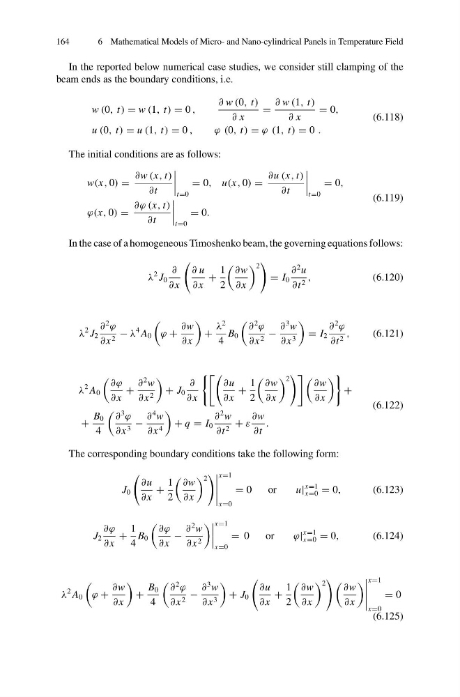
In the reported below numerical case studies, we consider still clamping of the
beam ends as the boundary conditions, i.e.
w (0, t) = w (1, t) = 0 ,
∂ w (0, t)
∂ x
=
∂ w (1, t)
∂ x
= 0,
u (0, t) = u (1, t) = 0 ,
ϕ (0, t) = ϕ (1, t) = 0 .
(6.118)
The initial conditions are as follows:
w(x, 0) =
∂w (x, t)
∂t
t=0
= 0, u(x, 0) =
∂u (x, t)
∂t
t=0
= 0,
ϕ(x, 0) =
∂ϕ (x, t)
∂t
t=0
= 0.
(6.119)
In the case of a homogeneous Timoshenko beam, the governing equations follows:
λ
2 J 0
∂
∂ x
∂ u
∂ x
+
1
2
∂w
∂ x
2
= I 0
∂
2 u
∂t 2 ,
(6.120)
λ
2 J 2
∂
2
ϕ
∂ x 2 − λ
4 A 0
ϕ +
∂w
∂ x
+
λ
2
4
B 0
∂
2
ϕ
∂ x 2 −
∂
3 w
∂ x 3
= I 2
∂
2
ϕ
∂t 2 ,
(6.121)
λ
2 A 0
∂ϕ
∂ x
+
∂
2 w
∂ x 2
+ J 0
∂
∂ x
∂u
∂ x
+
1
2
∂w
∂ x
2
∂w
∂ x
+
+
B 0
4
∂
3
ϕ
∂ x 3 −
∂
4 w
∂ x 4
+ q = I 0
∂
2 w
∂t 2 + ε
∂w
∂t
.
(6.122)
The corresponding boundary conditions take the following form:
J 0
∂u
∂ x
+
1
2
∂w
∂ x
2
x=1
x=0
= 0
or
u|
x=1
x=0 = 0,
(6.123)
J 2
∂ϕ
∂ x
+
1
4
B 0
∂ϕ
∂ x
−
∂
2 w
∂ x 2
x=1
x=0
= 0
or
ϕ|
x=1
x=0 = 0,
(6.124)
λ
2 A 0
ϕ +
∂w
∂ x
+
B 0
4
∂
2
ϕ
∂ x 2 −
∂
3 w
∂ x 3
+ J 0
∂u
∂ x
+
1
2
∂w
∂ x
2
∂w
∂ x
x=1
x=0
= 0
(6.125)
6 Mathematical Models of Micro- and Nano-cylindrical Panels in Temperature Field
In the reported below numerical case studies, we consider still clamping of the
beam ends as the boundary conditions, i.e.
w (0, t) = w (1, t) = 0 ,
∂ w (0, t)
∂ x
=
∂ w (1, t)
∂ x
= 0,
u (0, t) = u (1, t) = 0 ,
ϕ (0, t) = ϕ (1, t) = 0 .
(6.118)
The initial conditions are as follows:
w(x, 0) =
∂w (x, t)
∂t
t=0
= 0, u(x, 0) =
∂u (x, t)
∂t
t=0
= 0,
ϕ(x, 0) =
∂ϕ (x, t)
∂t
t=0
= 0.
(6.119)
In the case of a homogeneous Timoshenko beam, the governing equations follows:
λ
2 J 0
∂
∂ x
∂ u
∂ x
+
1
2
∂w
∂ x
2
= I 0
∂
2 u
∂t 2 ,
(6.120)
λ
2 J 2
∂
2
ϕ
∂ x 2 − λ
4 A 0
ϕ +
∂w
∂ x
+
λ
2
4
B 0
∂
2
ϕ
∂ x 2 −
∂
3 w
∂ x 3
= I 2
∂
2
ϕ
∂t 2 ,
(6.121)
λ
2 A 0
∂ϕ
∂ x
+
∂
2 w
∂ x 2
+ J 0
∂
∂ x
∂u
∂ x
+
1
2
∂w
∂ x
2
∂w
∂ x
+
+
B 0
4
∂
3
ϕ
∂ x 3 −
∂
4 w
∂ x 4
+ q = I 0
∂
2 w
∂t 2 + ε
∂w
∂t
.
(6.122)
The corresponding boundary conditions take the following form:
J 0
∂u
∂ x
+
1
2
∂w
∂ x
2
x=1
x=0
= 0
or
u|
x=1
x=0 = 0,
(6.123)
J 2
∂ϕ
∂ x
+
1
4
B 0
∂ϕ
∂ x
−
∂
2 w
∂ x 2
x=1
x=0
= 0
or
ϕ|
x=1
x=0 = 0,
(6.124)
λ
2 A 0
ϕ +
∂w
∂ x
+
B 0
4
∂
2
ϕ
∂ x 2 −
∂
3 w
∂ x 3
+ J 0
∂u
∂ x
+
1
2
∂w
∂ x
2
∂w
∂ x
x=1
x=0
= 0
(6.125)