

Kinematic Analysis and Simulation of Industrial Robot …
479
P y = a 3 ∗ (S 1 ∗ S 2 ∗ S 3 + C 2 ∗ C 3 ∗ S 1 )
− d 4 ∗ (C 2 ∗ S 1 ∗ S 3 − C 3 ∗ S 1 ∗ S 2 )
− d 2 ∗ C 1 + d 3 ∗ C 1 + a 1 ∗ S 1 + d 6
∗
S 5 ∗ (C 1 ∗ S 4 − C 4 ∗ (S 1 ∗ S 2 ∗ S 3 + C 2 ∗ C 3 ∗ S 1 ))
−C 5 ∗ (C 2 ∗ S 1 ∗ S 3 − C 3 ∗ S 1 ∗ S 2 )
+ a 2 ∗ C 2 ∗ S 1
(12)
P z = d 1 −
⎡
⎢
⎣
a 3 ∗ (C 2 ∗ S 3 − C 3 ∗ S 2 ) − d 4 ∗ (C 2 ∗ C 3 + S 2 ∗ S 3 )
− d 6 ∗ (C 5 ∗ (C 2 ∗ C 3 + S 2 ∗ S 3 ) − C 4 ∗ S 5 ∗ (C 2 ∗ S 3 − C 3 ∗ S 2 ))
+ a 2 ∗ S 2
⎤
⎥
⎦
(13)
where, C i denotes cosθ i , S i denotes sinθ i , C i *C j *S k = (cosθ i *cosθ j *sinθ k ). The
short notations of trigonometric identities makes the matrix compact and easy to
identify. The ‘R’ denotes the rotation elements of the end-effector in the spatial
workspace. Finally, the position of the end-effector, for the given joint variable vector
q = [θ 1 θ 2 θ 3 θ 4 θ 5 θ 6 ]
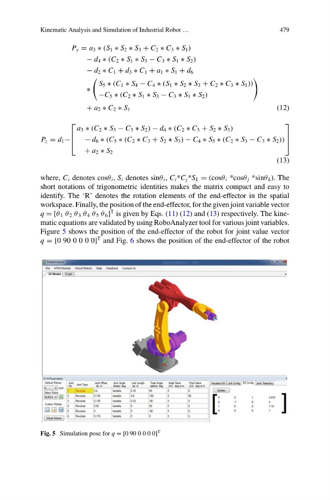
T is given by Eqs. (11) (12) and (13) respectively. The kinematic equations are validated by using RoboAnalyzer tool for various joint variables.
Figure 5 shows the position of the end-effector of the robot for joint value vector
q = [0 90 0 0 0 0]
T and Fig. 6 shows the position of the end-effector of the robot
Fig. 5 Simulation pose for q = [0 90 0 0 0 0] T
479
P y = a 3 ∗ (S 1 ∗ S 2 ∗ S 3 + C 2 ∗ C 3 ∗ S 1 )
− d 4 ∗ (C 2 ∗ S 1 ∗ S 3 − C 3 ∗ S 1 ∗ S 2 )
− d 2 ∗ C 1 + d 3 ∗ C 1 + a 1 ∗ S 1 + d 6
∗
S 5 ∗ (C 1 ∗ S 4 − C 4 ∗ (S 1 ∗ S 2 ∗ S 3 + C 2 ∗ C 3 ∗ S 1 ))
−C 5 ∗ (C 2 ∗ S 1 ∗ S 3 − C 3 ∗ S 1 ∗ S 2 )
+ a 2 ∗ C 2 ∗ S 1
(12)
P z = d 1 −
⎡
⎢
⎣
a 3 ∗ (C 2 ∗ S 3 − C 3 ∗ S 2 ) − d 4 ∗ (C 2 ∗ C 3 + S 2 ∗ S 3 )
− d 6 ∗ (C 5 ∗ (C 2 ∗ C 3 + S 2 ∗ S 3 ) − C 4 ∗ S 5 ∗ (C 2 ∗ S 3 − C 3 ∗ S 2 ))
+ a 2 ∗ S 2
⎤
⎥
⎦
(13)
where, C i denotes cosθ i , S i denotes sinθ i , C i *C j *S k = (cosθ i *cosθ j *sinθ k ). The
short notations of trigonometric identities makes the matrix compact and easy to
identify. The ‘R’ denotes the rotation elements of the end-effector in the spatial
workspace. Finally, the position of the end-effector, for the given joint variable vector
q = [θ 1 θ 2 θ 3 θ 4 θ 5 θ 6 ]
T is given by Eqs. (11) (12) and (13) respectively. The kinematic equations are validated by using RoboAnalyzer tool for various joint variables.
Figure 5 shows the position of the end-effector of the robot for joint value vector
q = [0 90 0 0 0 0]
T and Fig. 6 shows the position of the end-effector of the robot
Fig. 5 Simulation pose for q = [0 90 0 0 0 0] T