

478
A. Talli and A. C. Giriyapur
2 T 3 (θ 3 ) =
⎡
⎢
⎢
⎣
C 3 0 −S 3 a 3 ∗ C 3
S 3 0 C 3 a 3 ∗ S 3
0 −1 0
d 3
0 0 0
1
⎤
⎥
⎥
⎦
(4)
3 T 4 (θ 4 ) =
⎡
⎢
⎢
⎣
C 4 0 S 4 0
S 4 0 −C 4 0
0 1 0 d 4
0 0 0 1
⎤
⎥
⎥
⎦
(6)
4 T 5 (θ 5 ) =
⎡
⎢
⎢
⎣
C 5 0 −S 5 0
S 5 0 C 5 0
0 −1 0 0
0 0 0 1
⎤
⎥
⎥
⎦
(7)
5 T 6 (θ 6 ) =
⎡
⎢
⎢
⎣
C 6 −S 6 0 0
S 6 C 6 0 0
0 0 1 d 6
0 0 0 1
⎤
⎥
⎥
⎦
(8)
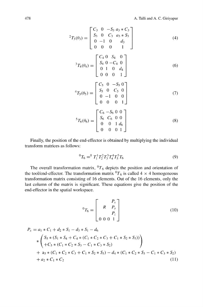
Finally, the position of the end-effector is obtained by multiplying the individual
transform matrices as follows:
0 T 6 =
0 T
1
1 T
2
2 T
3
3 T
4
4 T
5
5 T 6
(9)
The overall transformation matrix,
0 T 6 depicts the position and orientation of
the tool/end-effector. The transformation matrix
0 T 6 is called 4 × 4 homogeneous
transformation matrix consisting of 16 elements. Out of the 16 elements, only the
last column of the matrix is significant. These equations give the position of the
end-effector in the spatial workspace.
0 T 6 =
⎡
⎢
⎢
⎣
P x
R P y
P z
0 0 0 1
⎤
⎥
⎥
⎦
(10)
P x = a 1 ∗ C 1 + d 2 ∗ S 1 − d 3 ∗ S 1 − d 6
∗
S 5 ∗ (S 1 ∗ S 4 + C 4 ∗ (C 1 ∗ C 2 ∗ C 3 + C 1 ∗ S 2 ∗ S 3 ))
+C 5 ∗ (C 1 ∗ C 2 ∗ S 3 − C 1 ∗ C 3 ∗ S 2 )
+ a 3 ∗ (C 1 ∗ C 2 ∗ C 3 + C 1 ∗ S 2 ∗ S 3 ) − d 4 ∗ (C 1 ∗ C 2 ∗ S 3 − C 1 ∗ C 3 ∗ S 2 )
+ a 2 ∗ C 1 ∗ C 2
(11)
A. Talli and A. C. Giriyapur
2 T 3 (θ 3 ) =
⎡
⎢
⎢
⎣
C 3 0 −S 3 a 3 ∗ C 3
S 3 0 C 3 a 3 ∗ S 3
0 −1 0
d 3
0 0 0
1
⎤
⎥
⎥
⎦
(4)
3 T 4 (θ 4 ) =
⎡
⎢
⎢
⎣
C 4 0 S 4 0
S 4 0 −C 4 0
0 1 0 d 4
0 0 0 1
⎤
⎥
⎥
⎦
(6)
4 T 5 (θ 5 ) =
⎡
⎢
⎢
⎣
C 5 0 −S 5 0
S 5 0 C 5 0
0 −1 0 0
0 0 0 1
⎤
⎥
⎥
⎦
(7)
5 T 6 (θ 6 ) =
⎡
⎢
⎢
⎣
C 6 −S 6 0 0
S 6 C 6 0 0
0 0 1 d 6
0 0 0 1
⎤
⎥
⎥
⎦
(8)
Finally, the position of the end-effector is obtained by multiplying the individual
transform matrices as follows:
0 T 6 =
0 T
1
1 T
2
2 T
3
3 T
4
4 T
5
5 T 6
(9)
The overall transformation matrix,
0 T 6 depicts the position and orientation of
the tool/end-effector. The transformation matrix
0 T 6 is called 4 × 4 homogeneous
transformation matrix consisting of 16 elements. Out of the 16 elements, only the
last column of the matrix is significant. These equations give the position of the
end-effector in the spatial workspace.
0 T 6 =
⎡
⎢
⎢
⎣
P x
R P y
P z
0 0 0 1
⎤
⎥
⎥
⎦
(10)
P x = a 1 ∗ C 1 + d 2 ∗ S 1 − d 3 ∗ S 1 − d 6
∗
S 5 ∗ (S 1 ∗ S 4 + C 4 ∗ (C 1 ∗ C 2 ∗ C 3 + C 1 ∗ S 2 ∗ S 3 ))
+C 5 ∗ (C 1 ∗ C 2 ∗ S 3 − C 1 ∗ C 3 ∗ S 2 )
+ a 3 ∗ (C 1 ∗ C 2 ∗ C 3 + C 1 ∗ S 2 ∗ S 3 ) − d 4 ∗ (C 1 ∗ C 2 ∗ S 3 − C 1 ∗ C 3 ∗ S 2 )
+ a 2 ∗ C 1 ∗ C 2
(11)