

Estimation of Boundary Heat Flux with Conjugate …
347
The β
i is calculated by minimizing the Eq. (5a) with respect to β
i , that is,
min
β
i S
ˆ
q
i+1
(t)
=
min
β
i
t f
t=0
M
m=1
Y m (t) − T m
x meas , t; ˆ
q
i
(t) − β
i d
i
(t)
2 dt (5b)
The term T m
x meas , t; ˆ
q
i
(t) − β
i d
i
(t)
is evaluated by a Taylor expansion, Eq. (5b)
results in the linearized form
min
β
i S
ˆ
q
i+1
(t)
=
min
β
i
t f
t=0
M
m=1
Y m (t) − T m
x meas , t; ˆ
q
i
(t)
+β
i
T
x meas , t; d
i
(t)
2 dt
(5c)
where T
x meas , t; d
i
(t)
is obtain by solving the sensitivity problem given by
Eq. (4a), which is calculated by putting q
i (t) = d
i (t). Differentiate the Eq. (5c)
with respect to β
i and compare it with zero for minimization. Finally, we get the
following equation for β
i after doing some manipulation.
β
i
=
t f
t=0 T m
x meas , t; ˆ
q
i
(t)
− Y m (t)
T
x meas , t; d
i
(t)
dt
t f
t=0
T
x meas , t; d i (t)
2 dt
(6)
4.2 Adjoint Problem and Gradient Equation
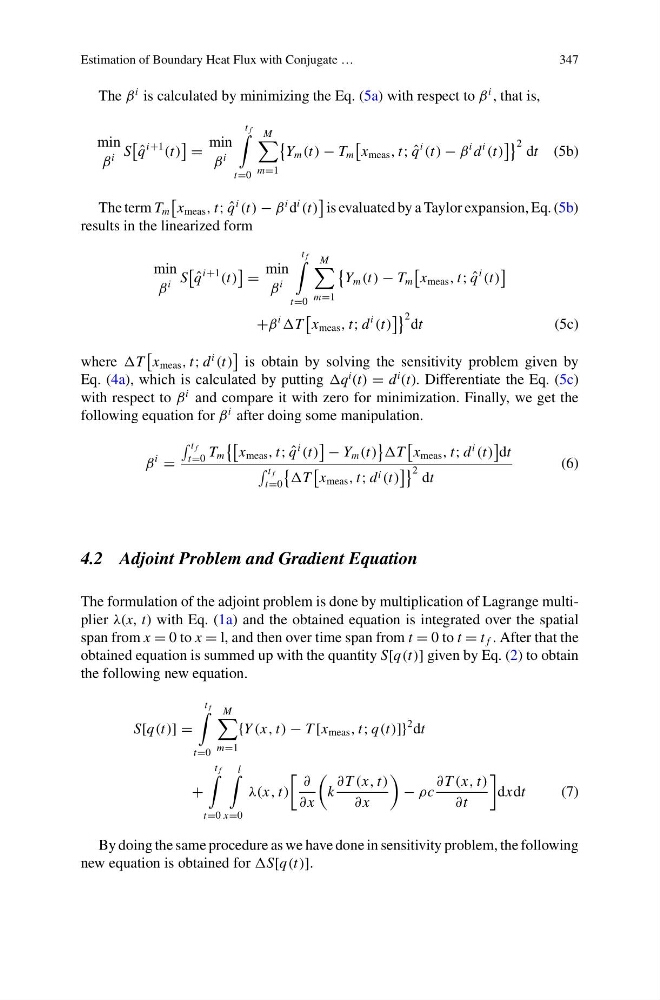
The formulation of the adjoint problem is done by multiplication of Lagrange multiplier λ(x, t) with Eq. (1a) and the obtained equation is integrated over the spatial
span from x = 0 to x = l, and then over time span from t = 0 to t = t f . After that the
obtained equation is summed up with the quantity S[q(t)] given by Eq. (2) to obtain
the following new equation.
S[q(t)] =
t f
t=0
M
m=1
{Y (x, t) − T [x meas , t; q(t)]}
2 dt
+
t f
t=0
l
x=0
λ(x, t)
∂
∂ x
k
∂ T (x, t)
∂ x
− ρc
∂ T (x, t)
∂t
dxdt
(7)
By doing the same procedure as we have done in sensitivity problem, the following
new equation is obtained for S[q(t)].
347
The β
i is calculated by minimizing the Eq. (5a) with respect to β
i , that is,
min
β
i S
ˆ
q
i+1
(t)
=
min
β
i
t f
t=0
M
m=1
Y m (t) − T m
x meas , t; ˆ
q
i
(t) − β
i d
i
(t)
2 dt (5b)
The term T m
x meas , t; ˆ
q
i
(t) − β
i d
i
(t)
is evaluated by a Taylor expansion, Eq. (5b)
results in the linearized form
min
β
i S
ˆ
q
i+1
(t)
=
min
β
i
t f
t=0
M
m=1
Y m (t) − T m
x meas , t; ˆ
q
i
(t)
+β
i
T
x meas , t; d
i
(t)
2 dt
(5c)
where T
x meas , t; d
i
(t)
is obtain by solving the sensitivity problem given by
Eq. (4a), which is calculated by putting q
i (t) = d
i (t). Differentiate the Eq. (5c)
with respect to β
i and compare it with zero for minimization. Finally, we get the
following equation for β
i after doing some manipulation.
β
i
=
t f
t=0 T m
x meas , t; ˆ
q
i
(t)
− Y m (t)
T
x meas , t; d
i
(t)
dt
t f
t=0
T
x meas , t; d i (t)
2 dt
(6)
4.2 Adjoint Problem and Gradient Equation
The formulation of the adjoint problem is done by multiplication of Lagrange multiplier λ(x, t) with Eq. (1a) and the obtained equation is integrated over the spatial
span from x = 0 to x = l, and then over time span from t = 0 to t = t f . After that the
obtained equation is summed up with the quantity S[q(t)] given by Eq. (2) to obtain
the following new equation.
S[q(t)] =
t f
t=0
M
m=1
{Y (x, t) − T [x meas , t; q(t)]}
2 dt
+
t f
t=0
l
x=0
λ(x, t)
∂
∂ x
k
∂ T (x, t)
∂ x
− ρc
∂ T (x, t)
∂t
dxdt
(7)
By doing the same procedure as we have done in sensitivity problem, the following
new equation is obtained for S[q(t)].