

348
P. Sathavara et al.
S[q(t)] =
t f
t=0
l
x=0
2{T [x meas , t; q(t)] − Y (x, t)}T (x, t)δ(x − x meas )dxdt
+
t f
t=0
l
x=0
λ(x, t)
∂
∂ x
k
∂∂T (x, t)
∂ x
− ρc
∂∂T (x, t)
∂t
dxdt
(8)
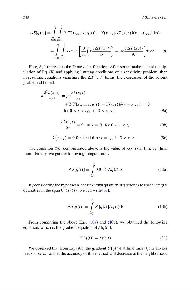
Here, δ(.) represents the Dirac delta function. After some mathematical manipulation of Eq. (8) and applying limiting conditions of a sensitivity problem, then
in resulting equations vanishing the T (x, t) terms, the expression of the adjoint
problem obtained:
k
∂
2
λ(x, t)
∂ x 2
= ρc
∂λ(x, t)
∂t
+ 2{T [x meas , t; q(t)] − Y (x, t)}δ(x − x meas ) = 0
for 0 < t < t f , in 0 < x < 1
( 9 a )
∂λ(0, t)
∂ x
= 0 at x = 0, for 0 < t < t f
(9b)
λ
x, t f
= 0 for final time t = t f , in 0 < x < 1
(9c)
The condition (9c) demonstrated above is the value of λ(x, t) at time t f (final
time). Finally, we get the following integral term:
S[q(t)] =
t f
t=0
λ(0, t)q(t)dt
(10a)
By considering the hypothesis, the unknown quantity q(t) belongs to space integral
quantities in the span 0 < t < t f , we can write[16]:
S[q(t)] =
t f
t=0
S
[q(t)]q(t)dt
(10b)
From comparing the above Eqs. (10a) and (10b), we obtained the following
equation, which is the gradient equation of S[q(t)].
S
[q(t)] = λ(0, t)
(11)
We observed that from Eq. (9c), the gradient S
[q(t)] at final time (t f ) is always
leads to zero, so that the accuracy of this method will decrease at the neighborhood
P. Sathavara et al.
S[q(t)] =
t f
t=0
l
x=0
2{T [x meas , t; q(t)] − Y (x, t)}T (x, t)δ(x − x meas )dxdt
+
t f
t=0
l
x=0
λ(x, t)
∂
∂ x
k
∂∂T (x, t)
∂ x
− ρc
∂∂T (x, t)
∂t
dxdt
(8)
Here, δ(.) represents the Dirac delta function. After some mathematical manipulation of Eq. (8) and applying limiting conditions of a sensitivity problem, then
in resulting equations vanishing the T (x, t) terms, the expression of the adjoint
problem obtained:
k
∂
2
λ(x, t)
∂ x 2
= ρc
∂λ(x, t)
∂t
+ 2{T [x meas , t; q(t)] − Y (x, t)}δ(x − x meas ) = 0
for 0 < t < t f , in 0 < x < 1
( 9 a )
∂λ(0, t)
∂ x
= 0 at x = 0, for 0 < t < t f
(9b)
λ
x, t f
= 0 for final time t = t f , in 0 < x < 1
(9c)
The condition (9c) demonstrated above is the value of λ(x, t) at time t f (final
time). Finally, we get the following integral term:
S[q(t)] =
t f
t=0
λ(0, t)q(t)dt
(10a)
By considering the hypothesis, the unknown quantity q(t) belongs to space integral
quantities in the span 0 < t < t f , we can write[16]:
S[q(t)] =
t f
t=0
S
[q(t)]q(t)dt
(10b)
From comparing the above Eqs. (10a) and (10b), we obtained the following
equation, which is the gradient equation of S[q(t)].
S
[q(t)] = λ(0, t)
(11)
We observed that from Eq. (9c), the gradient S
[q(t)] at final time (t f ) is always
leads to zero, so that the accuracy of this method will decrease at the neighborhood