

Estimation of Transient Boundary Heat Flux Using Modified JAYA …
335
where A W = ρ ∗C p∗ velocity * dy
A S = (k ∗ dx)/dy
B = q(t) ∗ dx
A P = A W + A S
For other points,
A P ∗ T P = A W ∗ T W + A S ∗ T S + A p0 ∗ T p0
(2.5)
where A W = ρ ∗C p∗ velocity * dy
A S = A N = (k ∗ dx)/dy
A P0 = (ρ ∗ dx ∗ dy)/dt
A P = A W + A S + A P0
To solve the convection term in governing equation, implicit upwind scheme is
used.
2.2 Inverse Problem
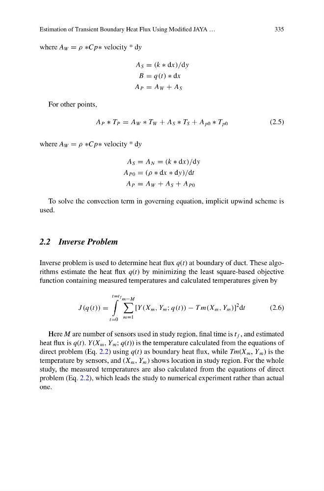
Inverse problem is used to determine heat flux q(t) at boundary of duct. These algorithms estimate the heat flux q(t) by minimizing the least square-based objective
function containing measured temperatures and calculated temperatures given by
J (q(t)) =
t=t f
t=0
m=M
m=1
[Y (X m , Y m ; q(t)) − T m(X m , Y m )]
2 dt
(2.6)
Here M are number of sensors used in study region, final time is t f , and estimated
heat flux is q(t). Y (X m , Y m ; q(t)) is the temperature calculated from the equations of
direct problem (Eq. 2.2) using q(t) as boundary heat flux, while Tm(X m , Y m ) is the
temperature by sensors, and (X m , Y m ) shows location in study region. For the whole
study, the measured temperatures are also calculated from the equations of direct
problem (Eq. 2.2), which leads the study to numerical experiment rather than actual
one.
335
where A W = ρ ∗C p∗ velocity * dy
A S = (k ∗ dx)/dy
B = q(t) ∗ dx
A P = A W + A S
For other points,
A P ∗ T P = A W ∗ T W + A S ∗ T S + A p0 ∗ T p0
(2.5)
where A W = ρ ∗C p∗ velocity * dy
A S = A N = (k ∗ dx)/dy
A P0 = (ρ ∗ dx ∗ dy)/dt
A P = A W + A S + A P0
To solve the convection term in governing equation, implicit upwind scheme is
used.
2.2 Inverse Problem
Inverse problem is used to determine heat flux q(t) at boundary of duct. These algorithms estimate the heat flux q(t) by minimizing the least square-based objective
function containing measured temperatures and calculated temperatures given by
J (q(t)) =
t=t f
t=0
m=M
m=1
[Y (X m , Y m ; q(t)) − T m(X m , Y m )]
2 dt
(2.6)
Here M are number of sensors used in study region, final time is t f , and estimated
heat flux is q(t). Y (X m , Y m ; q(t)) is the temperature calculated from the equations of
direct problem (Eq. 2.2) using q(t) as boundary heat flux, while Tm(X m , Y m ) is the
temperature by sensors, and (X m , Y m ) shows location in study region. For the whole
study, the measured temperatures are also calculated from the equations of direct
problem (Eq. 2.2), which leads the study to numerical experiment rather than actual
one.