

334
R. Prajapati et al.
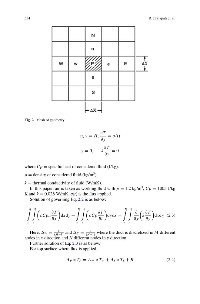
Fig. 2 Mesh of geometry
at, y = H,
∂ T
∂ y
= q(t)
y = 0, −k
∂ T
∂ y
= 0
where C p = specific heat of considered fluid (J/kg).
ρ = density of considered fluid (kg/m
3 ).
k = thermal conductivity of fluid (W/mK).
In this paper, air is taken as working fluid with ρ = 1.2 kg/m
3 , C p = 1005 J/kg
K and k = 0.026 W/mK. q(t) is the flux applied.
Solution of governing Eq. 2.2 is as below:
n
s
w
e
ρC pu
∂ T
∂ x
dxdy +
w
e
n
s
ρC p
∂ T
∂t
dydx =
w
e
n
s
∂
∂ y
k
∂ T
∂ y
dxdy (2.3)
Here, x =
b
(M−1)
and y =
h
(N −1)
where the duct is discretized in M different
nodes in x-direction and N different nodes in y-direction.
Further solution of Eq. 2.3 is as below.
For top surface where flux is applied,
A P ∗ T P = A W ∗ T W + A S ∗ T S + B
(2.4)
R. Prajapati et al.
Fig. 2 Mesh of geometry
at, y = H,
∂ T
∂ y
= q(t)
y = 0, −k
∂ T
∂ y
= 0
where C p = specific heat of considered fluid (J/kg).
ρ = density of considered fluid (kg/m
3 ).
k = thermal conductivity of fluid (W/mK).
In this paper, air is taken as working fluid with ρ = 1.2 kg/m
3 , C p = 1005 J/kg
K and k = 0.026 W/mK. q(t) is the flux applied.
Solution of governing Eq. 2.2 is as below:
n
s
w
e
ρC pu
∂ T
∂ x
dxdy +
w
e
n
s
ρC p
∂ T
∂t
dydx =
w
e
n
s
∂
∂ y
k
∂ T
∂ y
dxdy (2.3)
Here, x =
b
(M−1)
and y =
h
(N −1)
where the duct is discretized in M different
nodes in x-direction and N different nodes in y-direction.
Further solution of Eq. 2.3 is as below.
For top surface where flux is applied,
A P ∗ T P = A W ∗ T W + A S ∗ T S + B
(2.4)