

336
R. Prajapati et al.
2.2.1 Simple JAYA Algorithm
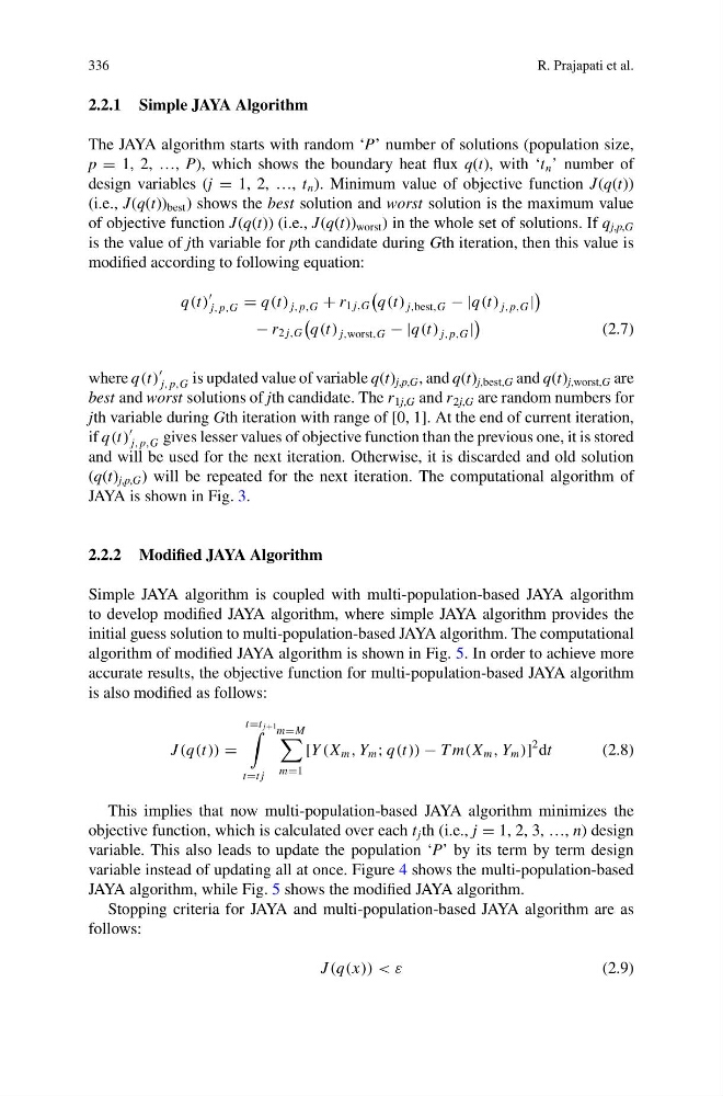
The JAYA algorithm starts with random ‘P’ number of solutions (population size,
p = 1, 2, …, P), which shows the boundary heat flux q(t), with ‘t n ’ number of
design variables (j = 1, 2, …, t n ). Minimum value of objective function J(q(t))
(i.e., J(q(t)) best ) shows the best solution and worst solution is the maximum value
of objective function J(q(t)) (i.e., J(q(t)) worst ) in the whole set of solutions. If q j,p,G
is the value of jth variable for pth candidate during Gth iteration, then this value is
modified according to following equation:
q(t)
j, p,G = q(t) j, p,G + r 1 j,G
q(t) j,best,G − |q(t) j, p,G |
− r 2 j,G
q(t) j,worst,G − |q(t) j, p,G |
(2.7)
where q(t)
j, p,G is updated value of variable q(t) j,p,G , and q(t) j,best,G and q(t) j,worst,G are
best and worst solutions of jth candidate. The r 1j,G and r 2j,G are random numbers for
jth variable during Gth iteration with range of [0, 1]. At the end of current iteration,
if q(t)
j, p,G gives lesser values of objective function than the previous one, it is stored
and will be used for the next iteration. Otherwise, it is discarded and old solution
(q(t) j,p,G ) will be repeated for the next iteration. The computational algorithm of
JAYA is shown in Fig. 3.
2.2.2 Modified JAYA Algorithm
Simple JAYA algorithm is coupled with multi-population-based JAYA algorithm
to develop modified JAYA algorithm, where simple JAYA algorithm provides the
initial guess solution to multi-population-based JAYA algorithm. The computational
algorithm of modified JAYA algorithm is shown in Fig. 5. In order to achieve more
accurate results, the objective function for multi-population-based JAYA algorithm
is also modified as follows:
J (q(t)) =
t=t j+1
t=t j
m=M
m=1
[Y (X m , Y m ; q(t)) − T m(X m , Y m )]
2 dt
(2.8)
This implies that now multi-population-based JAYA algorithm minimizes the
objective function, which is calculated over each t j th (i.e., j = 1, 2, 3, …, n) design
variable. This also leads to update the population ‘P’ by its term by term design
variable instead of updating all at once. Figure 4 shows the multi-population-based
JAYA algorithm, while Fig. 5 shows the modified JAYA algorithm.
Stopping criteria for JAYA and multi-population-based JAYA algorithm are as
follows:
J (q(x)) < ε
(2.9)
R. Prajapati et al.
2.2.1 Simple JAYA Algorithm
The JAYA algorithm starts with random ‘P’ number of solutions (population size,
p = 1, 2, …, P), which shows the boundary heat flux q(t), with ‘t n ’ number of
design variables (j = 1, 2, …, t n ). Minimum value of objective function J(q(t))
(i.e., J(q(t)) best ) shows the best solution and worst solution is the maximum value
of objective function J(q(t)) (i.e., J(q(t)) worst ) in the whole set of solutions. If q j,p,G
is the value of jth variable for pth candidate during Gth iteration, then this value is
modified according to following equation:
q(t)
j, p,G = q(t) j, p,G + r 1 j,G
q(t) j,best,G − |q(t) j, p,G |
− r 2 j,G
q(t) j,worst,G − |q(t) j, p,G |
(2.7)
where q(t)
j, p,G is updated value of variable q(t) j,p,G , and q(t) j,best,G and q(t) j,worst,G are
best and worst solutions of jth candidate. The r 1j,G and r 2j,G are random numbers for
jth variable during Gth iteration with range of [0, 1]. At the end of current iteration,
if q(t)
j, p,G gives lesser values of objective function than the previous one, it is stored
and will be used for the next iteration. Otherwise, it is discarded and old solution
(q(t) j,p,G ) will be repeated for the next iteration. The computational algorithm of
JAYA is shown in Fig. 3.
2.2.2 Modified JAYA Algorithm
Simple JAYA algorithm is coupled with multi-population-based JAYA algorithm
to develop modified JAYA algorithm, where simple JAYA algorithm provides the
initial guess solution to multi-population-based JAYA algorithm. The computational
algorithm of modified JAYA algorithm is shown in Fig. 5. In order to achieve more
accurate results, the objective function for multi-population-based JAYA algorithm
is also modified as follows:
J (q(t)) =
t=t j+1
t=t j
m=M
m=1
[Y (X m , Y m ; q(t)) − T m(X m , Y m )]
2 dt
(2.8)
This implies that now multi-population-based JAYA algorithm minimizes the
objective function, which is calculated over each t j th (i.e., j = 1, 2, 3, …, n) design
variable. This also leads to update the population ‘P’ by its term by term design
variable instead of updating all at once. Figure 4 shows the multi-population-based
JAYA algorithm, while Fig. 5 shows the modified JAYA algorithm.
Stopping criteria for JAYA and multi-population-based JAYA algorithm are as
follows:
J (q(x)) < ε
(2.9)