

Estimation of Thermodynamic and Transport Properties …
237
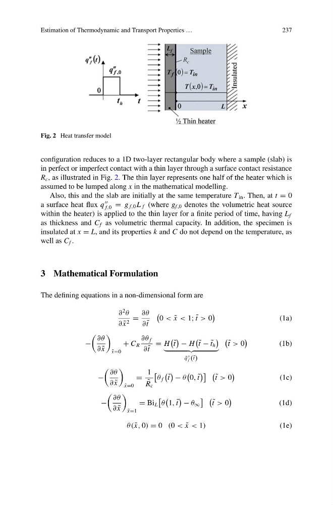
Fig. 2 Heat transfer model
configuration reduces to a 1D two-layer rectangular body where a sample (slab) is
in perfect or imperfect contact with a thin layer through a surface contact resistance
R c , as illustrated in Fig. 2. The thin layer represents one half of the heater which is
assumed to be lumped along x in the mathematical modelling.
Also, this and the slab are initially at the same temperature T in . Then, at t = 0
a surface heat flux q
f,0 = g f,0 L f (where g f ,0 denotes the volumetric heat source
within the heater) is applied to the thin layer for a finite period of time, having L f
as thickness and C f as volumetric thermal capacity. In addition, the specimen is
insulated at x = L, and its properties k and C do not depend on the temperature, as
well as C f .
3 Mathematical Formulation
The defining equations in a non-dimensional form are
∂
2
θ
∂ ˜
x 2 =
∂θ
∂ ˜
t
0 < ˜
x < 1; ˜
t > 0
(1a)
−
∂θ
∂ ˜
x
˜
x=0
+ C R
∂θ f
∂ ˜
t
= H
˜
t
− H
˜
t − ˜
t h
˜
q
f ( ˜
t)
˜
t > 0
(1b)
−
∂θ
∂ ˜
x
˜
x=0
=
1
˜
R c
θ f
˜
t
− θ
0, ˜
t
˜
t > 0
(1c)
−
∂θ
∂ ˜
x
˜
x=1
= Bi L
θ
1, ˜
t
− θ ∞
˜
t > 0
(1d)
θ ( ˜
x, 0) = 0 (0 < ˜
x < 1)
(1e)
237
Fig. 2 Heat transfer model
configuration reduces to a 1D two-layer rectangular body where a sample (slab) is
in perfect or imperfect contact with a thin layer through a surface contact resistance
R c , as illustrated in Fig. 2. The thin layer represents one half of the heater which is
assumed to be lumped along x in the mathematical modelling.
Also, this and the slab are initially at the same temperature T in . Then, at t = 0
a surface heat flux q
f,0 = g f,0 L f (where g f ,0 denotes the volumetric heat source
within the heater) is applied to the thin layer for a finite period of time, having L f
as thickness and C f as volumetric thermal capacity. In addition, the specimen is
insulated at x = L, and its properties k and C do not depend on the temperature, as
well as C f .
3 Mathematical Formulation
The defining equations in a non-dimensional form are
∂
2
θ
∂ ˜
x 2 =
∂θ
∂ ˜
t
0 < ˜
x < 1; ˜
t > 0
(1a)
−
∂θ
∂ ˜
x
˜
x=0
+ C R
∂θ f
∂ ˜
t
= H
˜
t
− H
˜
t − ˜
t h
˜
q
f ( ˜
t)
˜
t > 0
(1b)
−
∂θ
∂ ˜
x
˜
x=0
=
1
˜
R c
θ f
˜
t
− θ
0, ˜
t
˜
t > 0
(1c)
−
∂θ
∂ ˜
x
˜
x=1
= Bi L
θ
1, ˜
t
− θ ∞
˜
t > 0
(1d)
θ ( ˜
x, 0) = 0 (0 < ˜
x < 1)
(1e)