

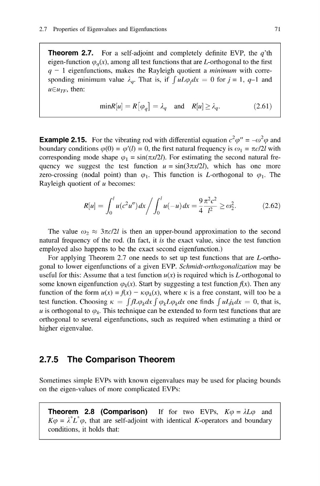
Theorem 2.7. For a self-adjoint and completely definite EVP, the q’th
eigen-function u q (x), among all test functions that are L-orthogonal to the first
q − 1 eigenfunctions, makes the Rayleigh quotient a minimum with corresponding minimum value k q . That is, if
R
uLu j dx ¼ 0 for j = 1, q–1 and
u2u TF , then:
minR u
½ ¼ R u q
 à ¼ k q and R u
½ ! k q :
ð2:61Þ
Example 2.15. For the vibrating rod with differential equation c
2 u′′ = –x
2 u and
boundary conditions u(0) = u′(l) = 0, the first natural frequency is x 1 = pc/2l with
corresponding mode shape u 1 = sin(px/2l). For estimating the second natural frequency we suggest the test function u = sin(3px/2l), which has one more
zero-crossing (nodal point) than u 1 . This function is L-orthogonal to u 1 . The
Rayleigh quotient of u becomes:
R u
½ ¼
Z l
0
uðc
2 u
00
Þ dx
0Z l
0
uðÀuÞdx ¼
9
4
p
2 c
2
l 2 ! x
2
2 :
ð2:62Þ
The value x 2 % 3pc/2l is then an upper-bound approximation to the second
natural frequency of the rod. (In fact, it is the exact value, since the test function
employed also happens to be the exact second eigenfunction.)
For applying Theorem 2.7 one needs to set up test functions that are L-orthogonal to lower eigenfunctions of a given EVP. Schmidt-orthogonalization may be
useful for this: Assume that a test function u(x) is required which is L-orthogonal to
some known eigenfunction u k (x). Start by suggesting a test function f(x). Then any
function of the form u(x) = f(x) − ju k (x), where j is a free constant, will too be a
test function. Choosing j ¼
R
fLu k dx
R
u k Lu k dx one finds
R
uLj k dx ¼ 0, that is,
u is orthogonal to u k . This technique can be extended to form test functions that are
orthogonal to several eigenfunctions, such as required when estimating a third or
higher eigenvalue.
2.7.5 The Comparison Theorem
Sometimes simple EVPs with known eigenvalues may be used for placing bounds
on the eigen-values of more complicated EVPs:
Theorem 2.8 (Comparison)
If for two EVPs, Ku = kLu and
Ku = k
* L
* u, that are self-adjoint with identical K-operators and boundary
conditions, it holds that:
2.7 Properties of Eigenvalues and Eigenfunctions
71
eigen-function u q (x), among all test functions that are L-orthogonal to the first
q − 1 eigenfunctions, makes the Rayleigh quotient a minimum with corresponding minimum value k q . That is, if
R
uLu j dx ¼ 0 for j = 1, q–1 and
u2u TF , then:
minR u
½ ¼ R u q
 à ¼ k q and R u
½ ! k q :
ð2:61Þ
Example 2.15. For the vibrating rod with differential equation c
2 u′′ = –x
2 u and
boundary conditions u(0) = u′(l) = 0, the first natural frequency is x 1 = pc/2l with
corresponding mode shape u 1 = sin(px/2l). For estimating the second natural frequency we suggest the test function u = sin(3px/2l), which has one more
zero-crossing (nodal point) than u 1 . This function is L-orthogonal to u 1 . The
Rayleigh quotient of u becomes:
R u
½ ¼
Z l
0
uðc
2 u
00
Þ dx
0Z l
0
uðÀuÞdx ¼
9
4
p
2 c
2
l 2 ! x
2
2 :
ð2:62Þ
The value x 2 % 3pc/2l is then an upper-bound approximation to the second
natural frequency of the rod. (In fact, it is the exact value, since the test function
employed also happens to be the exact second eigenfunction.)
For applying Theorem 2.7 one needs to set up test functions that are L-orthogonal to lower eigenfunctions of a given EVP. Schmidt-orthogonalization may be
useful for this: Assume that a test function u(x) is required which is L-orthogonal to
some known eigenfunction u k (x). Start by suggesting a test function f(x). Then any
function of the form u(x) = f(x) − ju k (x), where j is a free constant, will too be a
test function. Choosing j ¼
R
fLu k dx
R
u k Lu k dx one finds
R
uLj k dx ¼ 0, that is,
u is orthogonal to u k . This technique can be extended to form test functions that are
orthogonal to several eigenfunctions, such as required when estimating a third or
higher eigenvalue.
2.7.5 The Comparison Theorem
Sometimes simple EVPs with known eigenvalues may be used for placing bounds
on the eigen-values of more complicated EVPs:
Theorem 2.8 (Comparison)
If for two EVPs, Ku = kLu and
Ku = k
* L
* u, that are self-adjoint with identical K-operators and boundary
conditions, it holds that:
2.7 Properties of Eigenvalues and Eigenfunctions
71