

d 00 ¼ À
1
2
e
2
þ Oðe
3
Þ;
d 1À ¼ 1 À
ffiffiffiffiffiffiffiffiffiffiffiffiffiffiffiffiffi
e 2 À 4l 2
p
À
1
8
e
2
þ Oðe
3
Þ;
d 1 þ ¼ 1 þ
ffiffiffiffiffiffiffiffiffiffiffiffiffiffiffiffiffi
e 2 À 4l 2
p
À
1
8
e
2
þ Oðe
3
Þ;
d 4À ¼ 4 þ
1
6
e
2
À
ffiffiffiffiffiffiffiffiffiffiffiffiffiffiffiffiffiffiffiffiffiffiffi
1
16
e 4 À 16l 2
r
þ Oðe
3
Þ;
d 4 þ ¼ 4 þ
1
6
e
2
þ
ffiffiffiffiffiffiffiffiffiffiffiffiffiffiffiffiffiffiffiffiffiffiffi
1
16
e 4 À 16l 2
r
þ Oðe
3
Þ;
ðC:13Þ
which are valid for l ( 1 and e ( 1, to the order of magnitude indicated.
A damped Mathieu equation can be transformed into the undamped standard
form (C.11). For example, the variable shift uðsÞ ! uðsÞ expðÀlsÞ transforms
(C.12) into the form (C.11) (where d then changes to d − l
2 ).
Similarly, the equation of motion for a linear single-degree-of-freedom oscillator
with parametric excitation typically takes this form:
€ x þ 2b_ x þ x
2
þ q cosðXtÞ
À
Á
x ¼ 0;
ðC:14Þ
where x = x(t) and ð
:
Þ ¼ d=dt. To transform this into the undamped standard form
(C.11), we first introduce a new independent variable s =
1
2 Xt (to get the argument
of the cosine right), and then introduce a new dependent variable u by letting x
(s) = u(s)exp(cs). Inserting this into (C.14), it is found that the damping term
vanishes by choosing c = –2b /X, and that the undamped form (C.11) then is
obtained with the following values of d and e:
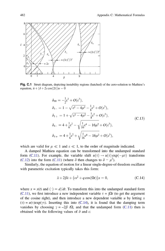
Fig. C.1 Strutt diagram, depicting instability regions (hatched) of the zero-solution to Mathieu’s
equation, € u þ d þ 2e cosð2tÞ
ð
Þ u ¼ 0
482
Appendix C: Mathematical Formulas
1
2
e
2
þ Oðe
3
Þ;
d 1À ¼ 1 À
ffiffiffiffiffiffiffiffiffiffiffiffiffiffiffiffiffi
e 2 À 4l 2
p
À
1
8
e
2
þ Oðe
3
Þ;
d 1 þ ¼ 1 þ
ffiffiffiffiffiffiffiffiffiffiffiffiffiffiffiffiffi
e 2 À 4l 2
p
À
1
8
e
2
þ Oðe
3
Þ;
d 4À ¼ 4 þ
1
6
e
2
À
ffiffiffiffiffiffiffiffiffiffiffiffiffiffiffiffiffiffiffiffiffiffiffi
1
16
e 4 À 16l 2
r
þ Oðe
3
Þ;
d 4 þ ¼ 4 þ
1
6
e
2
þ
ffiffiffiffiffiffiffiffiffiffiffiffiffiffiffiffiffiffiffiffiffiffiffi
1
16
e 4 À 16l 2
r
þ Oðe
3
Þ;
ðC:13Þ
which are valid for l ( 1 and e ( 1, to the order of magnitude indicated.
A damped Mathieu equation can be transformed into the undamped standard
form (C.11). For example, the variable shift uðsÞ ! uðsÞ expðÀlsÞ transforms
(C.12) into the form (C.11) (where d then changes to d − l
2 ).
Similarly, the equation of motion for a linear single-degree-of-freedom oscillator
with parametric excitation typically takes this form:
€ x þ 2b_ x þ x
2
þ q cosðXtÞ
À
Á
x ¼ 0;
ðC:14Þ
where x = x(t) and ð
:
Þ ¼ d=dt. To transform this into the undamped standard form
(C.11), we first introduce a new independent variable s =
1
2 Xt (to get the argument
of the cosine right), and then introduce a new dependent variable u by letting x
(s) = u(s)exp(cs). Inserting this into (C.14), it is found that the damping term
vanishes by choosing c = –2b /X, and that the undamped form (C.11) then is
obtained with the following values of d and e:
Fig. C.1 Strutt diagram, depicting instability regions (hatched) of the zero-solution to Mathieu’s
equation, € u þ d þ 2e cosð2tÞ
ð
Þ u ¼ 0
482
Appendix C: Mathematical Formulas