

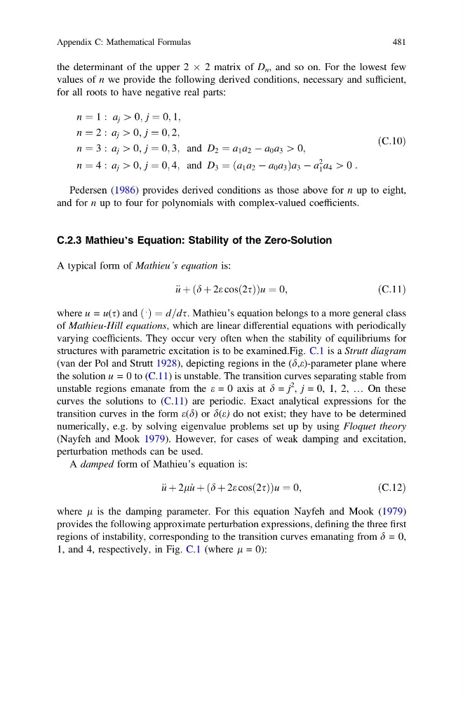
the determinant of the upper 2 Â 2 matrix of D n , and so on. For the lowest few
values of n we provide the following derived conditions, necessary and sufficient,
for all roots to have negative real parts:
n ¼ 1 : a j [ 0; j ¼ 0; 1;
n ¼ 2 : a j [ 0; j ¼ 0; 2;
n ¼ 3 : a j [ 0; j ¼ 0; 3; and D 2 ¼ a 1 a 2 À a 0 a 3 [ 0;
n ¼ 4 : a j [ 0; j ¼ 0; 4; and D 3 ¼ a 1 a 2 À a 0 a 3
ð
Þ a 3 À a
2
1 a 4 [ 0 :
ðC:10Þ
Pedersen (1986) provides derived conditions as those above for n up to eight,
and for n up to four for polynomials with complex-valued coefficients.
C.2.3 Mathieu’s Equation: Stability of the Zero-Solution
A typical form of Mathieu’s equation is:
€ u þ d þ 2e cosð2sÞ
ð
Þ u ¼ 0;
ðC:11Þ
where u = u(s) and ð
:
Þ ¼ d=ds. Mathieu’s equation belongs to a more general class
of Mathieu-Hill equations, which are linear differential equations with periodically
varying coefficients. They occur very often when the stability of equilibriums for
structures with parametric excitation is to be examined.Fig. C.1 is a Strutt diagram
(van der Pol and Strutt 1928), depicting regions in the (d,e)-parameter plane where
the solution u = 0 to (C.11) is unstable. The transition curves separating stable from
unstable regions emanate from the e = 0 axis at d = j
2 , j = 0, 1, 2, … On these
curves the solutions to (C.11) are periodic. Exact analytical expressions for the
transition curves in the form e(d) or d(e) do not exist; they have to be determined
numerically, e.g. by solving eigenvalue problems set up by using Floquet theory
(Nayfeh and Mook 1979). However, for cases of weak damping and excitation,
perturbation methods can be used.
A damped form of Mathieu’s equation is:
€ u þ 2l _
u þ d þ 2e cosð2sÞ
ð
Þ u ¼ 0;
ðC:12Þ
where l is the damping parameter. For this equation Nayfeh and Mook (1979)
provides the following approximate perturbation expressions, defining the three first
regions of instability, corresponding to the transition curves emanating from d = 0,
1, and 4, respectively, in Fig. C.1 (where l = 0):
Appendix C: Mathematical Formulas
481
values of n we provide the following derived conditions, necessary and sufficient,
for all roots to have negative real parts:
n ¼ 1 : a j [ 0; j ¼ 0; 1;
n ¼ 2 : a j [ 0; j ¼ 0; 2;
n ¼ 3 : a j [ 0; j ¼ 0; 3; and D 2 ¼ a 1 a 2 À a 0 a 3 [ 0;
n ¼ 4 : a j [ 0; j ¼ 0; 4; and D 3 ¼ a 1 a 2 À a 0 a 3
ð
Þ a 3 À a
2
1 a 4 [ 0 :
ðC:10Þ
Pedersen (1986) provides derived conditions as those above for n up to eight,
and for n up to four for polynomials with complex-valued coefficients.
C.2.3 Mathieu’s Equation: Stability of the Zero-Solution
A typical form of Mathieu’s equation is:
€ u þ d þ 2e cosð2sÞ
ð
Þ u ¼ 0;
ðC:11Þ
where u = u(s) and ð
:
Þ ¼ d=ds. Mathieu’s equation belongs to a more general class
of Mathieu-Hill equations, which are linear differential equations with periodically
varying coefficients. They occur very often when the stability of equilibriums for
structures with parametric excitation is to be examined.Fig. C.1 is a Strutt diagram
(van der Pol and Strutt 1928), depicting regions in the (d,e)-parameter plane where
the solution u = 0 to (C.11) is unstable. The transition curves separating stable from
unstable regions emanate from the e = 0 axis at d = j
2 , j = 0, 1, 2, … On these
curves the solutions to (C.11) are periodic. Exact analytical expressions for the
transition curves in the form e(d) or d(e) do not exist; they have to be determined
numerically, e.g. by solving eigenvalue problems set up by using Floquet theory
(Nayfeh and Mook 1979). However, for cases of weak damping and excitation,
perturbation methods can be used.
A damped form of Mathieu’s equation is:
€ u þ 2l _
u þ d þ 2e cosð2sÞ
ð
Þ u ¼ 0;
ðC:12Þ
where l is the damping parameter. For this equation Nayfeh and Mook (1979)
provides the following approximate perturbation expressions, defining the three first
regions of instability, corresponding to the transition curves emanating from d = 0,
1, and 4, respectively, in Fig. C.1 (where l = 0):
Appendix C: Mathematical Formulas
481