

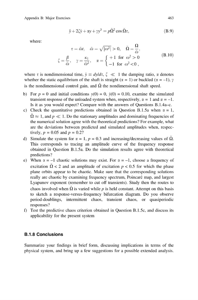
€ y þ 2f_ y þ ay þ cy
3
¼ p ~
X
2 cos ~
Xs;
ðB:9Þ
where:
s ¼ ~
xt; ~
x ¼
ffiffiffiffiffiffiffiffi
x 2
j j
p
[ 0; ~
X ¼
X
~
x
;
f ¼
b
~
x
; c ¼
j 1
~
x 2 ; a ¼
þ 1 for x
2
[ 0
À1 for x
2
\0 ;
&
ðB:10Þ
where s is nondimensional time, _
y dy/ds, f ( 1 the damping ratio, a denotes
whether the static equilibrium of the shaft is straight (a = 1) or buckled (a = –1), c
is the nondimensional control gain, and ~
X the nondimensional shaft speed.
b) For p = 0 and initial conditions y(0) = 0, _
y(0) = 0.10, examine the simulated
transient response of the unloaded system when, respectively, a = 1 and a = –1.
Is it as you would expect? Compare with the answers of Questions B.1.4a–c.
c) Check the quantitative predictions obtained in Question B.1.5a when a = 1,
~
X % 1, and p ( 1. Do the stationary amplitudes and dominating frequencies of
the numerical solution agree with the theoretical predictions? For example, what
are the deviations between predicted and simulated amplitudes when, respectively, p = 0.05 and p = 0.2?
d) Simulate the system for a = 1, p = 0.3 and increasing/decreasing values of ~
X.
This corresponds to tracing an amplitude curve of the frequency response
obtained in Question B.1.5a. Do the simulation results agree with theoretical
predictions?
e) When a = –1 chaotic solutions may exist. For a = –1, choose a frequency of
excitation ~
X < 2 and an amplitude of excitation p < 0.5 for which the phase
plane orbits appear to be chaotic. Make sure that the corresponding solutions
really are chaotic by examining frequency spectrum, Poincaré map, and largest
Lyapunov exponent (remember to cut off transients). Study then the routes to
chaos involved when ~
X is varied while p is held constant. Attempt on this basis
to sketch a response-versus-frequency bifurcation diagram. Do you observe
period-doublings, intermittent chaos, transient chaos, or quasiperiodic
responses?
f) Test the predictive chaos criterion obtained in Question B.1.5c, and discuss its
applicability for the present system
B.1.8 Conclusions
Summarize your findings in brief form, discussing implications in terms of the
physical system, and bring up a few suggestions for a possible extended analysis.
Appendix B: Major Exercises
463
3
¼ p ~
X
2 cos ~
Xs;
ðB:9Þ
where:
s ¼ ~
xt; ~
x ¼
ffiffiffiffiffiffiffiffi
x 2
j j
p
[ 0; ~
X ¼
X
~
x
;
f ¼
b
~
x
; c ¼
j 1
~
x 2 ; a ¼
þ 1 for x
2
[ 0
À1 for x
2
\0 ;
&
ðB:10Þ
where s is nondimensional time, _
y dy/ds, f ( 1 the damping ratio, a denotes
whether the static equilibrium of the shaft is straight (a = 1) or buckled (a = –1), c
is the nondimensional control gain, and ~
X the nondimensional shaft speed.
b) For p = 0 and initial conditions y(0) = 0, _
y(0) = 0.10, examine the simulated
transient response of the unloaded system when, respectively, a = 1 and a = –1.
Is it as you would expect? Compare with the answers of Questions B.1.4a–c.
c) Check the quantitative predictions obtained in Question B.1.5a when a = 1,
~
X % 1, and p ( 1. Do the stationary amplitudes and dominating frequencies of
the numerical solution agree with the theoretical predictions? For example, what
are the deviations between predicted and simulated amplitudes when, respectively, p = 0.05 and p = 0.2?
d) Simulate the system for a = 1, p = 0.3 and increasing/decreasing values of ~
X.
This corresponds to tracing an amplitude curve of the frequency response
obtained in Question B.1.5a. Do the simulation results agree with theoretical
predictions?
e) When a = –1 chaotic solutions may exist. For a = –1, choose a frequency of
excitation ~
X < 2 and an amplitude of excitation p < 0.5 for which the phase
plane orbits appear to be chaotic. Make sure that the corresponding solutions
really are chaotic by examining frequency spectrum, Poincaré map, and largest
Lyapunov exponent (remember to cut off transients). Study then the routes to
chaos involved when ~
X is varied while p is held constant. Attempt on this basis
to sketch a response-versus-frequency bifurcation diagram. Do you observe
period-doublings, intermittent chaos, transient chaos, or quasiperiodic
responses?
f) Test the predictive chaos criterion obtained in Question B.1.5c, and discuss its
applicability for the present system
B.1.8 Conclusions
Summarize your findings in brief form, discussing implications in terms of the
physical system, and bring up a few suggestions for a possible extended analysis.
Appendix B: Major Exercises
463