

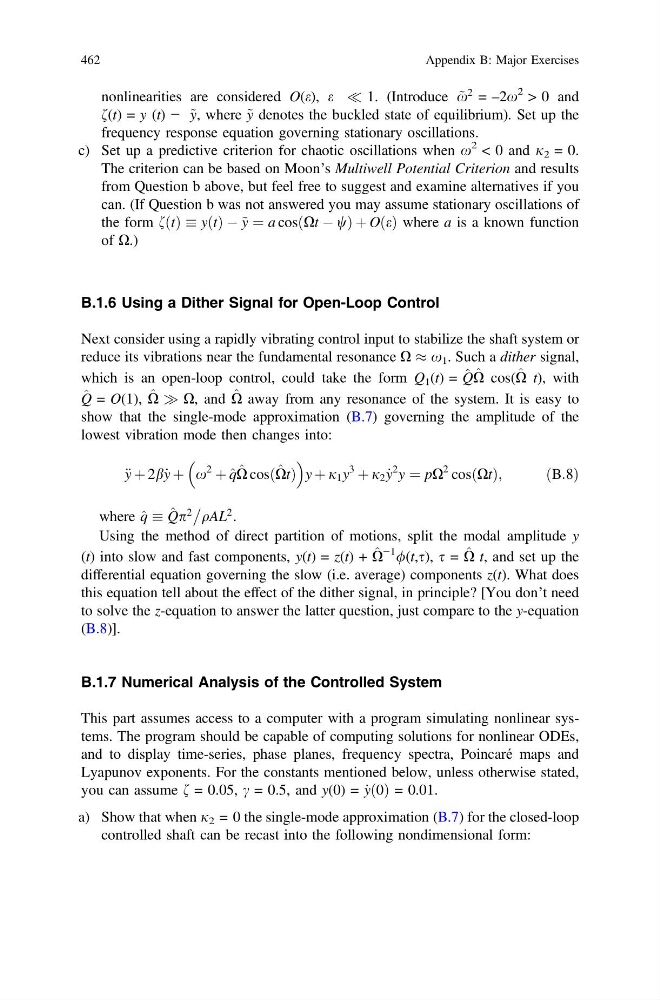
nonlinearities are considered O(e), e ( 1. (Introduce ~
x
2 = –2x
2 > 0 and
f(t) = y (t) − ~ y, where ~ y denotes the buckled state of equilibrium). Set up the
frequency response equation governing stationary oscillations.
c) Set up a predictive criterion for chaotic oscillations when x
2 < 0 and j 2 = 0.
The criterion can be based on Moon’s Multiwell Potential Criterion and results
from Question b above, but feel free to suggest and examine alternatives if you
can. (If Question b was not answered you may assume stationary oscillations of
the form fðtÞ yðtÞ À ~ y ¼ a cosðXt À wÞ þ OðeÞ where a is a known function
of X.)
B.1.6 Using a Dither Signal for Open-Loop Control
Next consider using a rapidly vibrating control input to stabilize the shaft system or
reduce its vibrations near the fundamental resonance X % x 1 . Such a dither signal,
which is an open-loop control, could take the form Q 1 (t) = ^
Q ^
X cos( ^
X t), with
^
Q = O(1), ^
X ) X, and ^
X away from any resonance of the system. It is easy to
show that the single-mode approximation (B.7) governing the amplitude of the
lowest vibration mode then changes into:
€ y þ 2b_ y þ x
2
þ ^ q ^
X cosð ^
XtÞ
y þ j 1 y
3
þ j 2 _
y
2 y ¼ pX
2 cosðXtÞ;
ðB:8Þ
where ^ q ^
Qp
2
qAL
2 .
Using the method of direct partition of motions, split the modal amplitude y
(t) into slow and fast components, y(t) = z(t) + ^
X
−1 /(t,s), s = ^
X t, and set up the
differential equation governing the slow (i.e. average) components z(t). What does
this equation tell about the effect of the dither signal, in principle? [You don’t need
to solve the z-equation to answer the latter question, just compare to the y-equation
(B.8)].
B.1.7 Numerical Analysis of the Controlled System
This part assumes access to a computer with a program simulating nonlinear systems. The program should be capable of computing solutions for nonlinear ODEs,
and to display time-series, phase planes, frequency spectra, Poincaré maps and
Lyapunov exponents. For the constants mentioned below, unless otherwise stated,
you can assume f = 0.05, c = 0.5, and y(0) = _
yð0Þ = 0.01.
a) Show that when j 2 = 0 the single-mode approximation (B.7) for the closed-loop
controlled shaft can be recast into the following nondimensional form:
462
Appendix B: Major Exercises
x
2 = –2x
2 > 0 and
f(t) = y (t) − ~ y, where ~ y denotes the buckled state of equilibrium). Set up the
frequency response equation governing stationary oscillations.
c) Set up a predictive criterion for chaotic oscillations when x
2 < 0 and j 2 = 0.
The criterion can be based on Moon’s Multiwell Potential Criterion and results
from Question b above, but feel free to suggest and examine alternatives if you
can. (If Question b was not answered you may assume stationary oscillations of
the form fðtÞ yðtÞ À ~ y ¼ a cosðXt À wÞ þ OðeÞ where a is a known function
of X.)
B.1.6 Using a Dither Signal for Open-Loop Control
Next consider using a rapidly vibrating control input to stabilize the shaft system or
reduce its vibrations near the fundamental resonance X % x 1 . Such a dither signal,
which is an open-loop control, could take the form Q 1 (t) = ^
Q ^
X cos( ^
X t), with
^
Q = O(1), ^
X ) X, and ^
X away from any resonance of the system. It is easy to
show that the single-mode approximation (B.7) governing the amplitude of the
lowest vibration mode then changes into:
€ y þ 2b_ y þ x
2
þ ^ q ^
X cosð ^
XtÞ
y þ j 1 y
3
þ j 2 _
y
2 y ¼ pX
2 cosðXtÞ;
ðB:8Þ
where ^ q ^
Qp
2
qAL
2 .
Using the method of direct partition of motions, split the modal amplitude y
(t) into slow and fast components, y(t) = z(t) + ^
X
−1 /(t,s), s = ^
X t, and set up the
differential equation governing the slow (i.e. average) components z(t). What does
this equation tell about the effect of the dither signal, in principle? [You don’t need
to solve the z-equation to answer the latter question, just compare to the y-equation
(B.8)].
B.1.7 Numerical Analysis of the Controlled System
This part assumes access to a computer with a program simulating nonlinear systems. The program should be capable of computing solutions for nonlinear ODEs,
and to display time-series, phase planes, frequency spectra, Poincaré maps and
Lyapunov exponents. For the constants mentioned below, unless otherwise stated,
you can assume f = 0.05, c = 0.5, and y(0) = _
yð0Þ = 0.01.
a) Show that when j 2 = 0 the single-mode approximation (B.7) for the closed-loop
controlled shaft can be recast into the following nondimensional form:
462
Appendix B: Major Exercises