

v
f;m
¼
X
k;j
n
0
k n
0
j
D
E
rf j M
À1
f k þ
M
À1
f k
À
Á T rM ð1Þ M
À1
f l
. .
.
M
À1
f k
À
Á T rM ðnÞ M
À1
f l
8
> <
> :
9
> =
> ;
0
B
B
@
1
C
C
A
u¼z¼0
: ð7:91Þ
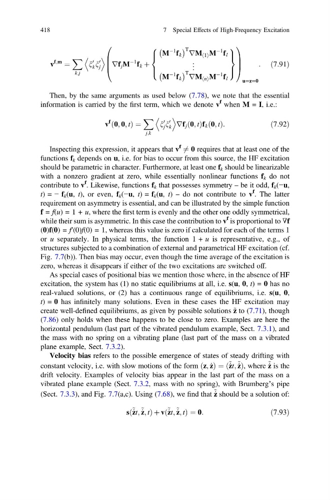
Then, by the same arguments as used below (7.78), we note that the essential
information is carried by the first term, which we denote v
f when M = I, i.e.:
v
f
ð0; 0; tÞ ¼
X
j;k
n
0
j n
0
k
D
E
rf j ð0; tÞf k ð0; tÞ:
ð7:92Þ
Inspecting this expression, it appears that v
f
6 ¼ 0 requires that at least one of the
functions f k depends on u, i.e. for bias to occur from this source, the HF excitation
should be parametric in character. Furthermore, at least one f k should be linearizable
with a nonzero gradient at zero, while essentially nonlinear functions f k do not
contribute to v
f . Likewise, functions f k that possesses symmetry – be it odd, f k (−u,
t) = − f k (u, t), or even, f k (−u, t) = f k (u, t) – do not contribute to v
f
. The latter
requirement on asymmetry is essential, and can be illustrated by the simple function
f = f(u) = 1 + u, where the first term is evenly and the other one oddly symmetrical,
while their sum is asymmetric. In this case the contribution to v
f is proportional to ∇f
(0)f(0) = f′(0)f(0) = 1, whereas this value is zero if calculated for each of the terms 1
or u separately. In physical terms, the function 1 + u is representative, e.g., of
structures subjected to a combination of external and parametrical HF excitation (cf.
Fig. 7.7(b)). Then bias may occur, even though the time average of the excitation is
zero, whereas it disappears if either of the two excitations are switched off.
As special cases of positional bias we mention those where, in the absence of HF
excitation, the system has (1) no static equilibriums at all, i.e. s(u, 0, t) = 0 has no
real-valued solutions, or (2) has a continuous range of equilibriums, i.e. s(u, 0,
t) = 0 has infinitely many solutions. Even in these cases the HF excitation may
create well-defined equilibriums, as given by possible solutions ~ z to (7.71), though
(7.86) only holds when these happens to be close to zero. Examples are here the
horizontal pendulum (last part of the vibrated pendulum example, Sect. 7.3.1), and
the mass with no spring on a vibrating plane (last part of the mass on a vibrated
plane example, Sect. 7.3.2).
Velocity bias refers to the possible emergence of states of steady drifting with
constant velocity, i.e. with slow motions of the form ðz; _
zÞ ¼ ð ~ _
zt; ~ _
zÞ, where ~ _
z is the
drift velocity. Examples of velocity bias appear in the last part of the mass on a
vibrated plane example (Sect. 7.3.2, mass with no spring), with Brumberg’s pipe
(Sect. 7.3.3), and Fig. 7.7(a,c). Using (7.68), we find that ~ _
z should be a solution of:
sð ~ _
zt; ~ _
z; tÞ þ vð ~ _
zt; ~ _
z; tÞ ¼ 0:
ð7:93Þ
418
7 Special Effects of High-Frequency Excitation
f;m
¼
X
k;j
n
0
k n
0
j
D
E
rf j M
À1
f k þ
M
À1
f k
À
Á T rM ð1Þ M
À1
f l
. .
.
M
À1
f k
À
Á T rM ðnÞ M
À1
f l
8
> <
> :
9
> =
> ;
0
B
B
@
1
C
C
A
u¼z¼0
: ð7:91Þ
Then, by the same arguments as used below (7.78), we note that the essential
information is carried by the first term, which we denote v
f when M = I, i.e.:
v
f
ð0; 0; tÞ ¼
X
j;k
n
0
j n
0
k
D
E
rf j ð0; tÞf k ð0; tÞ:
ð7:92Þ
Inspecting this expression, it appears that v
f
6 ¼ 0 requires that at least one of the
functions f k depends on u, i.e. for bias to occur from this source, the HF excitation
should be parametric in character. Furthermore, at least one f k should be linearizable
with a nonzero gradient at zero, while essentially nonlinear functions f k do not
contribute to v
f . Likewise, functions f k that possesses symmetry – be it odd, f k (−u,
t) = − f k (u, t), or even, f k (−u, t) = f k (u, t) – do not contribute to v
f
. The latter
requirement on asymmetry is essential, and can be illustrated by the simple function
f = f(u) = 1 + u, where the first term is evenly and the other one oddly symmetrical,
while their sum is asymmetric. In this case the contribution to v
f is proportional to ∇f
(0)f(0) = f′(0)f(0) = 1, whereas this value is zero if calculated for each of the terms 1
or u separately. In physical terms, the function 1 + u is representative, e.g., of
structures subjected to a combination of external and parametrical HF excitation (cf.
Fig. 7.7(b)). Then bias may occur, even though the time average of the excitation is
zero, whereas it disappears if either of the two excitations are switched off.
As special cases of positional bias we mention those where, in the absence of HF
excitation, the system has (1) no static equilibriums at all, i.e. s(u, 0, t) = 0 has no
real-valued solutions, or (2) has a continuous range of equilibriums, i.e. s(u, 0,
t) = 0 has infinitely many solutions. Even in these cases the HF excitation may
create well-defined equilibriums, as given by possible solutions ~ z to (7.71), though
(7.86) only holds when these happens to be close to zero. Examples are here the
horizontal pendulum (last part of the vibrated pendulum example, Sect. 7.3.1), and
the mass with no spring on a vibrating plane (last part of the mass on a vibrated
plane example, Sect. 7.3.2).
Velocity bias refers to the possible emergence of states of steady drifting with
constant velocity, i.e. with slow motions of the form ðz; _
zÞ ¼ ð ~ _
zt; ~ _
zÞ, where ~ _
z is the
drift velocity. Examples of velocity bias appear in the last part of the mass on a
vibrated plane example (Sect. 7.3.2, mass with no spring), with Brumberg’s pipe
(Sect. 7.3.3), and Fig. 7.7(a,c). Using (7.68), we find that ~ _
z should be a solution of:
sð ~ _
zt; ~ _
z; tÞ þ vð ~ _
zt; ~ _
z; tÞ ¼ 0:
ð7:93Þ
418
7 Special Effects of High-Frequency Excitation