

7.5.2 Example Functions
For the example systems in Sect. 7.3 one has, for the pendulum with a vibrating
support: u = h, M = 1, s ¼ 2b _
h + sinh, m = 1, h 1 = 0, f 1 = −qXsinh, n 1 = −
sinXt; for the mass on a vibrating plane: u = u, M = 1, s = x
2 u +
l sgn( _
u) + l D ,
m = 1, h 1 = 0, f 1 = −qX, n = −sinXt; and for Brumberg’s pipe: u = x, M = 1,
s = 1, m = 2, h 1 = 0, f 1 = −a x X, n 1 = sin(2Xt), h 2 = −la y X
2 sgn(_ x), f 2 = 0, n 2 = |
sin(Xt)| − 2/p.
7.5.3 The Averaged System Governing the ‘Slow’
Motions
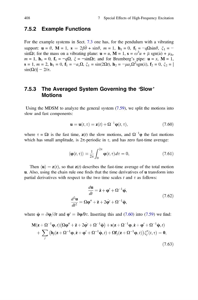
Using the MDSM to analyze the general system (7.59), we split the motions into
slow and fast components:
u ¼ uðt; sÞ ¼ zðtÞ þ X
À1
uðt; sÞ;
ð7:60Þ
where s = Xt is the fast time, z(t) the slow motions, and X
−1
φ the fast motions
which has small amplitude, is 2p-periodic in s, and has zero fast-time average:
uðt; sÞ
h
i
1
2p
Z 2p
0
uðt; sÞds ¼ 0;
ð7:61Þ
Then u
h i ¼ zðtÞ, so that z(t) describes the fast-time average of the total motion
u. Also, using the chain rule one finds that the time derivatives of u transform into
partial derivatives with respect to the two time scales t and s as follows:
du
dt
¼ _
z þ u
0
þ X
À1
_
u;
d
2
u
dt 2 ¼ Xu
00
þ € z þ 2 _
u 0 þ X
À1
€
u;
ð7:62Þ
where _
u @u=@t and φ′ ∂φ/∂s. Inserting this and (7.60) into (7.59) we find:
Mðz þ X
À1
u; tÞ Xu
00
þ € z þ 2 _
u 0 þ X
À1
€
u
À
Á þ sðz þ X
À1
u; _
z þ u
0
þ X
À1
_
u; tÞ
þ
X
j
h j ðz þ X
À1
u; _
z þ u
0
þ X
À1
_
u; tÞ þ Xf j ðz þ X
À1
u; tÞ
À
Á
n
00
j ðt; sÞ ¼ 0;
ð7:63Þ
408
7 Special Effects of High-Frequency Excitation
For the example systems in Sect. 7.3 one has, for the pendulum with a vibrating
support: u = h, M = 1, s ¼ 2b _
h + sinh, m = 1, h 1 = 0, f 1 = −qXsinh, n 1 = −
sinXt; for the mass on a vibrating plane: u = u, M = 1, s = x
2 u +
l sgn( _
u) + l D ,
m = 1, h 1 = 0, f 1 = −qX, n = −sinXt; and for Brumberg’s pipe: u = x, M = 1,
s = 1, m = 2, h 1 = 0, f 1 = −a x X, n 1 = sin(2Xt), h 2 = −la y X
2 sgn(_ x), f 2 = 0, n 2 = |
sin(Xt)| − 2/p.
7.5.3 The Averaged System Governing the ‘Slow’
Motions
Using the MDSM to analyze the general system (7.59), we split the motions into
slow and fast components:
u ¼ uðt; sÞ ¼ zðtÞ þ X
À1
uðt; sÞ;
ð7:60Þ
where s = Xt is the fast time, z(t) the slow motions, and X
−1
φ the fast motions
which has small amplitude, is 2p-periodic in s, and has zero fast-time average:
uðt; sÞ
h
i
1
2p
Z 2p
0
uðt; sÞds ¼ 0;
ð7:61Þ
Then u
h i ¼ zðtÞ, so that z(t) describes the fast-time average of the total motion
u. Also, using the chain rule one finds that the time derivatives of u transform into
partial derivatives with respect to the two time scales t and s as follows:
du
dt
¼ _
z þ u
0
þ X
À1
_
u;
d
2
u
dt 2 ¼ Xu
00
þ € z þ 2 _
u 0 þ X
À1
€
u;
ð7:62Þ
where _
u @u=@t and φ′ ∂φ/∂s. Inserting this and (7.60) into (7.59) we find:
Mðz þ X
À1
u; tÞ Xu
00
þ € z þ 2 _
u 0 þ X
À1
€
u
À
Á þ sðz þ X
À1
u; _
z þ u
0
þ X
À1
_
u; tÞ
þ
X
j
h j ðz þ X
À1
u; _
z þ u
0
þ X
À1
_
u; tÞ þ Xf j ðz þ X
À1
u; tÞ
À
Á
n
00
j ðt; sÞ ¼ 0;
ð7:63Þ
408
7 Special Effects of High-Frequency Excitation