

Again we determine approximate solutions for the case of high excitation frequency X ) x and small excitation amplitude q ( 1, by splitting motions into
slow and fast components:
x ¼ xðt; sÞ ¼ zðtÞ þ X
À1 uðt; sÞ;
ð7:36Þ
where z holds the slow motions, X
−1
φ is a small overlay of zero average fast
motions, and s = Xt is the fast time scale. Proceeding as for the pendulum example
in the previous section we find that the fast motions are:
uðt; sÞ ¼ ÀqX sin s þ OðX
À1
Þ;
ð7:37Þ
while the slow motions are governed by:
€ z þ x
2 z þ
l sgn _
z À qX cos s
ð
Þ
h
i þ l D ¼ 0;
ð7:38Þ
where hi denotes the averaging operator defined by (7.20) or (7.5). Hence, by (7.36)
and (7.37), motions of the mass are given by:
xðtÞ ¼ zðtÞ À q sinðXtÞ þ OðX
À2
Þ:
ð7:39Þ
The average term in (7.38) can be calculated by noting that the argument of the
signum function is positive for s2[s 1 ;s 2 ] where t 1 ¼ arccosð_ z=qXÞ and s 2 = 2p − s 1 ,
and otherwise negative. As a result the equation of slow motions becomes:
€ z þ x
2 z þ f ð_ zÞ ¼ 0;
ð7:40Þ
where f is the effective friction force:
f ð_ zÞ ¼
lsgnð_ zÞ þ l D
for _
z
j j ! qX;
l 1 À
2
p arccos _
z=qX
ð
Þ
ð
Þ þ l D for _
z
j j\qX:
&
ð7:41Þ
Comparing to the original Eq. (7.34) for x, it appears that the non-autonomous
excitation term has disappeared, and that the term representing friction force has
changed for velocities _
z
j j\qX.
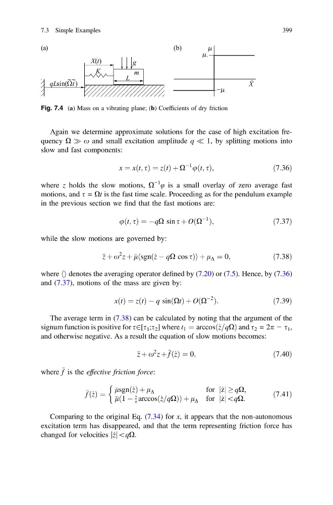
Fig. 7.4 (a) Mass on a vibrating plane; (b) Coefficients of dry friction
7.3 Simple Examples
399
slow and fast components:
x ¼ xðt; sÞ ¼ zðtÞ þ X
À1 uðt; sÞ;
ð7:36Þ
where z holds the slow motions, X
−1
φ is a small overlay of zero average fast
motions, and s = Xt is the fast time scale. Proceeding as for the pendulum example
in the previous section we find that the fast motions are:
uðt; sÞ ¼ ÀqX sin s þ OðX
À1
Þ;
ð7:37Þ
while the slow motions are governed by:
€ z þ x
2 z þ
l sgn _
z À qX cos s
ð
Þ
h
i þ l D ¼ 0;
ð7:38Þ
where hi denotes the averaging operator defined by (7.20) or (7.5). Hence, by (7.36)
and (7.37), motions of the mass are given by:
xðtÞ ¼ zðtÞ À q sinðXtÞ þ OðX
À2
Þ:
ð7:39Þ
The average term in (7.38) can be calculated by noting that the argument of the
signum function is positive for s2[s 1 ;s 2 ] where t 1 ¼ arccosð_ z=qXÞ and s 2 = 2p − s 1 ,
and otherwise negative. As a result the equation of slow motions becomes:
€ z þ x
2 z þ f ð_ zÞ ¼ 0;
ð7:40Þ
where f is the effective friction force:
f ð_ zÞ ¼
lsgnð_ zÞ þ l D
for _
z
j j ! qX;
l 1 À
2
p arccos _
z=qX
ð
Þ
ð
Þ þ l D for _
z
j j\qX:
&
ð7:41Þ
Comparing to the original Eq. (7.34) for x, it appears that the non-autonomous
excitation term has disappeared, and that the term representing friction force has
changed for velocities _
z
j j\qX.
Fig. 7.4 (a) Mass on a vibrating plane; (b) Coefficients of dry friction
7.3 Simple Examples
399