

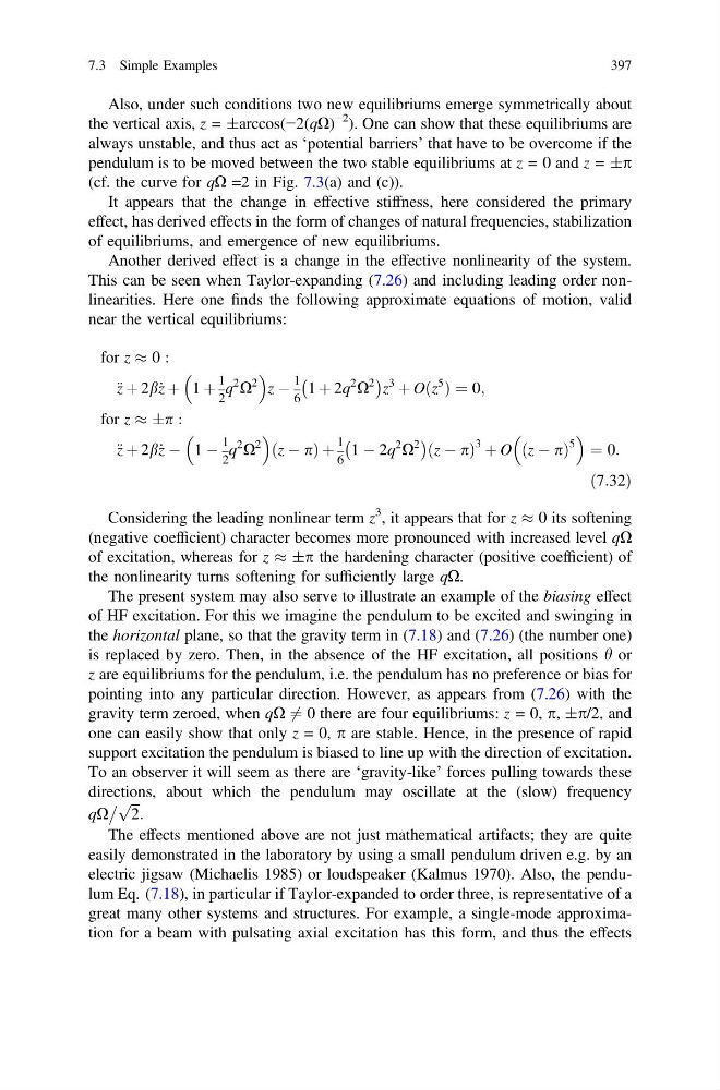
Also, under such conditions two new equilibriums emerge symmetrically about
the vertical axis, z = ±arccos(−2(qX)
−2 ). One can show that these equilibriums are
always unstable, and thus act as ‘potential barriers’ that have to be overcome if the
pendulum is to be moved between the two stable equilibriums at z = 0 and z = ±p
(cf. the curve for qX =2 in Fig. 7.3(a) and (c)).
It appears that the change in effective stiffness, here considered the primary
effect, has derived effects in the form of changes of natural frequencies, stabilization
of equilibriums, and emergence of new equilibriums.
Another derived effect is a change in the effective nonlinearity of the system.
This can be seen when Taylor-expanding (7.26) and including leading order nonlinearities. Here one finds the following approximate equations of motion, valid
near the vertical equilibriums:
for z % 0 :
€ z þ 2b_ z þ 1 þ
1
2
q
2
X
2
z À
1
6
1 þ 2q
2
X
2
À
Á
z
3
þ Oðz
5
Þ ¼ 0;
for z % Æp :
€ z þ 2b_ z À 1 À
1
2
q
2
X
2
ðz À pÞ þ
1
6
1 À 2q
2
X
2
À
Á
ðz À pÞ
3 þ O ðz À pÞ
5
¼ 0:
ð7:32Þ
Considering the leading nonlinear term z
3 , it appears that for z % 0 its softening
(negative coefficient) character becomes more pronounced with increased level qX
of excitation, whereas for z % ±p the hardening character (positive coefficient) of
the nonlinearity turns softening for sufficiently large qX.
The present system may also serve to illustrate an example of the biasing effect
of HF excitation. For this we imagine the pendulum to be excited and swinging in
the horizontal plane, so that the gravity term in (7.18) and (7.26) (the number one)
is replaced by zero. Then, in the absence of the HF excitation, all positions h or
z are equilibriums for the pendulum, i.e. the pendulum has no preference or bias for
pointing into any particular direction. However, as appears from (7.26) with the
gravity term zeroed, when qX 6 ¼ 0 there are four equilibriums: z = 0, p, ±p/2, and
one can easily show that only z = 0, p are stable. Hence, in the presence of rapid
support excitation the pendulum is biased to line up with the direction of excitation.
To an observer it will seem as there are ‘gravity-like’ forces pulling towards these
directions, about which the pendulum may oscillate at the (slow) frequency
qX
ffiffi ffi
2
p :
The effects mentioned above are not just mathematical artifacts; they are quite
easily demonstrated in the laboratory by using a small pendulum driven e.g. by an
electric jigsaw (Michaelis 1985) or loudspeaker (Kalmus 1970). Also, the pendulum Eq. (7.18), in particular if Taylor-expanded to order three, is representative of a
great many other systems and structures. For example, a single-mode approximation for a beam with pulsating axial excitation has this form, and thus the effects
7.3 Simple Examples
397
the vertical axis, z = ±arccos(−2(qX)
−2 ). One can show that these equilibriums are
always unstable, and thus act as ‘potential barriers’ that have to be overcome if the
pendulum is to be moved between the two stable equilibriums at z = 0 and z = ±p
(cf. the curve for qX =2 in Fig. 7.3(a) and (c)).
It appears that the change in effective stiffness, here considered the primary
effect, has derived effects in the form of changes of natural frequencies, stabilization
of equilibriums, and emergence of new equilibriums.
Another derived effect is a change in the effective nonlinearity of the system.
This can be seen when Taylor-expanding (7.26) and including leading order nonlinearities. Here one finds the following approximate equations of motion, valid
near the vertical equilibriums:
for z % 0 :
€ z þ 2b_ z þ 1 þ
1
2
q
2
X
2
z À
1
6
1 þ 2q
2
X
2
À
Á
z
3
þ Oðz
5
Þ ¼ 0;
for z % Æp :
€ z þ 2b_ z À 1 À
1
2
q
2
X
2
ðz À pÞ þ
1
6
1 À 2q
2
X
2
À
Á
ðz À pÞ
3 þ O ðz À pÞ
5
¼ 0:
ð7:32Þ
Considering the leading nonlinear term z
3 , it appears that for z % 0 its softening
(negative coefficient) character becomes more pronounced with increased level qX
of excitation, whereas for z % ±p the hardening character (positive coefficient) of
the nonlinearity turns softening for sufficiently large qX.
The present system may also serve to illustrate an example of the biasing effect
of HF excitation. For this we imagine the pendulum to be excited and swinging in
the horizontal plane, so that the gravity term in (7.18) and (7.26) (the number one)
is replaced by zero. Then, in the absence of the HF excitation, all positions h or
z are equilibriums for the pendulum, i.e. the pendulum has no preference or bias for
pointing into any particular direction. However, as appears from (7.26) with the
gravity term zeroed, when qX 6 ¼ 0 there are four equilibriums: z = 0, p, ±p/2, and
one can easily show that only z = 0, p are stable. Hence, in the presence of rapid
support excitation the pendulum is biased to line up with the direction of excitation.
To an observer it will seem as there are ‘gravity-like’ forces pulling towards these
directions, about which the pendulum may oscillate at the (slow) frequency
qX
ffiffi ffi
2
p :
The effects mentioned above are not just mathematical artifacts; they are quite
easily demonstrated in the laboratory by using a small pendulum driven e.g. by an
electric jigsaw (Michaelis 1985) or loudspeaker (Kalmus 1970). Also, the pendulum Eq. (7.18), in particular if Taylor-expanded to order three, is representative of a
great many other systems and structures. For example, a single-mode approximation for a beam with pulsating axial excitation has this form, and thus the effects
7.3 Simple Examples
397