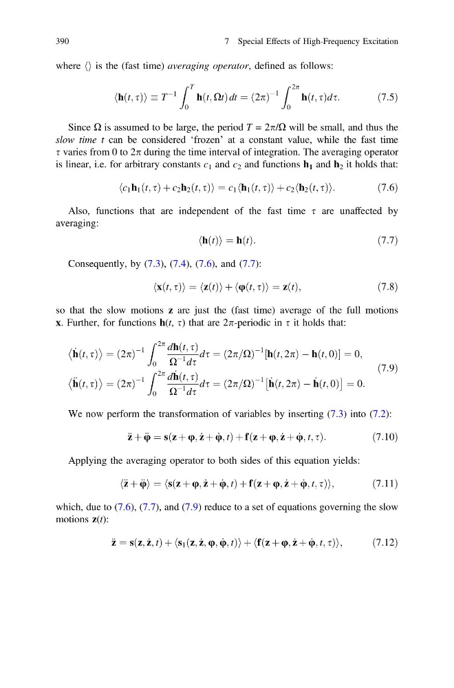
where hi is the (fast time) averaging operator, defined as follows:
hðt; sÞ
h
i T
À1
Z T
0
hðt; XtÞdt ¼ ð2pÞ
À1
Z 2p
0
hðt; sÞds:
ð7:5Þ
Since X is assumed to be large, the period T = 2p/X will be small, and thus the
slow time t can be considered ‘frozen’ at a constant value, while the fast time
s varies from 0 to 2p during the time interval of integration. The averaging operator
is linear, i.e. for arbitrary constants c 1 and c 2 and functions h 1 and h 2 it holds that:
c 1 h 1 ðt; sÞ þ c 2 h 2 ðt; sÞ
h
i ¼ c 1 h 1 ðt; sÞ
h
iþ c 2 h 2 ðt; sÞ
h
i:
ð7:6Þ
Also, functions that are independent of the fast time s are unaffected by
averaging:
hðtÞ
h
i ¼ hðtÞ:
ð7:7Þ
Consequently, by (7.3), (7.4), (7.6), and (7.7):
xðt; sÞ
h
i¼ zðtÞ
h
iþ uðt; sÞ
h
i¼ zðtÞ;
ð7:8Þ
so that the slow motions z are just the (fast time) average of the full motions
x. Further, for functions h(t, s) that are 2p-periodic in s it holds that:
_
hðt; sÞ
¼ ð2pÞ
À1
Z 2p
0
dhðt; sÞ
X
À1 ds
ds ¼ ð2p=XÞ
À1 hðt; 2pÞ À hðt; 0Þ
½
Š ¼ 0;
€
hðt; sÞ
¼ ð2pÞ
À1
Z 2p
0
d _
hðt; sÞ
X
À1 ds
ds ¼ ð2p=XÞ
À1 _
hðt; 2pÞ À _
hðt; 0Þ
Â
à ¼ 0:
ð7:9Þ
We now perform the transformation of variables by inserting (7.3) into (7.2):
€ z þ €
u ¼ sðz þ u; _
z þ _
u; tÞ þ fðz þ u; _
z þ _
u; t; sÞ:
ð7:10Þ
Applying the averaging operator to both sides of this equation yields:
€ z þ €
u
h
i¼ sðz þ u; _
z þ _
u; tÞ þ fðz þ u; _
z þ _
u; t; sÞ
h
i ;
ð7:11Þ
which, due to (7.6), (7.7), and (7.9) reduce to a set of equations governing the slow
motions z(t):
€ z ¼ sðz; _
z; tÞ þ s 1 ðz; _
z; u; _
u; tÞ
h
i þ fðz þ u; _
z þ _
u; t; sÞ
h
i ;
ð7:12Þ
390
7 Special Effects of High-Frequency Excitation