

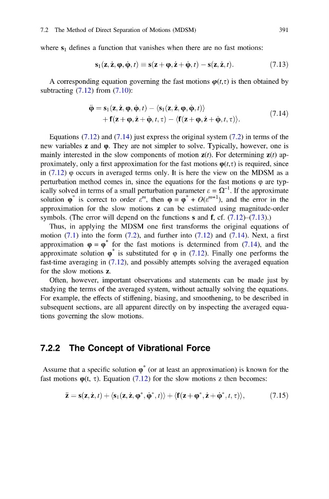
where s 1 defines a function that vanishes when there are no fast motions:
s 1 ðz; _
z; u; _
u; tÞ sðz þ u; _
z þ _
u; tÞ À sðz; _
z; tÞ:
ð7:13Þ
A corresponding equation governing the fast motions u(t,s) is then obtained by
subtracting (7.12) from (7.10):
€
u ¼ s 1 ðz; _
z; u; _
u; tÞ À s 1 ðz; _
z; u; _
u; tÞ
h
i
þ fðz þ u; _
z þ _
u; t; sÞ À fðz þ u; _
z þ _
u; t; sÞ
h
i :
ð7:14Þ
Equations (7.12) and (7.14) just express the original system (7.2) in terms of the
new variables z and φ. They are not simpler to solve. Typically, however, one is
mainly interested in the slow components of motion z(t). For determining z(t) approximately, only a first approximation for the fast motions φ(t,s) is required, since
in (7.12) φ occurs in averaged terms only. It is here the view on the MDSM as a
perturbation method comes in, since the equations for the fast motions φ are typically solved in terms of a small perturbation parameter e = X
–1 . If the approximate
solution φ
* is correct to order e
m , then φ = φ
* + O(e
m+1 ), and the error in the
approximation for the slow motions z can be estimated using magnitude-order
symbols. (The error will depend on the functions s and f, cf. (7.12)–(7.13).)
Thus, in applying the MDSM one first transforms the original equations of
motion (7.1) into the form (7.2), and further into (7.12) and (7.14). Next, a first
approximation φ = φ
* for the fast motions is determined from (7.14), and the
approximate solution φ
* is substituted for φ in (7.12). Finally one performs the
fast-time averaging in (7.12), and possibly attempts solving the averaged equation
for the slow motions z.
Often, however, important observations and statements can be made just by
studying the terms of the averaged system, without actually solving the equations.
For example, the effects of stiffening, biasing, and smoothening, to be described in
subsequent sections, are all apparent directly on by inspecting the averaged equations governing the slow motions.
7.2.2 The Concept of Vibrational Force
Assume that a specific solution φ
* (or at least an approximation) is known for the
fast motions φ(t, s). Equation (7.12) for the slow motions z then becomes:
€ z ¼ sðz; _
z; tÞ þ s 1 ðz; _
z; u
Ã
; _
u
Ã
; tÞ
h
i þ fðz þ u
Ã
; _
z þ _
u
Ã
; t; sÞ
h
i ;
ð7:15Þ
7.2 The Method of Direct Separation of Motions (MDSM)
391
s 1 ðz; _
z; u; _
u; tÞ sðz þ u; _
z þ _
u; tÞ À sðz; _
z; tÞ:
ð7:13Þ
A corresponding equation governing the fast motions u(t,s) is then obtained by
subtracting (7.12) from (7.10):
€
u ¼ s 1 ðz; _
z; u; _
u; tÞ À s 1 ðz; _
z; u; _
u; tÞ
h
i
þ fðz þ u; _
z þ _
u; t; sÞ À fðz þ u; _
z þ _
u; t; sÞ
h
i :
ð7:14Þ
Equations (7.12) and (7.14) just express the original system (7.2) in terms of the
new variables z and φ. They are not simpler to solve. Typically, however, one is
mainly interested in the slow components of motion z(t). For determining z(t) approximately, only a first approximation for the fast motions φ(t,s) is required, since
in (7.12) φ occurs in averaged terms only. It is here the view on the MDSM as a
perturbation method comes in, since the equations for the fast motions φ are typically solved in terms of a small perturbation parameter e = X
–1 . If the approximate
solution φ
* is correct to order e
m , then φ = φ
* + O(e
m+1 ), and the error in the
approximation for the slow motions z can be estimated using magnitude-order
symbols. (The error will depend on the functions s and f, cf. (7.12)–(7.13).)
Thus, in applying the MDSM one first transforms the original equations of
motion (7.1) into the form (7.2), and further into (7.12) and (7.14). Next, a first
approximation φ = φ
* for the fast motions is determined from (7.14), and the
approximate solution φ
* is substituted for φ in (7.12). Finally one performs the
fast-time averaging in (7.12), and possibly attempts solving the averaged equation
for the slow motions z.
Often, however, important observations and statements can be made just by
studying the terms of the averaged system, without actually solving the equations.
For example, the effects of stiffening, biasing, and smoothening, to be described in
subsequent sections, are all apparent directly on by inspecting the averaged equations governing the slow motions.
7.2.2 The Concept of Vibrational Force
Assume that a specific solution φ
* (or at least an approximation) is known for the
fast motions φ(t, s). Equation (7.12) for the slow motions z then becomes:
€ z ¼ sðz; _
z; tÞ þ s 1 ðz; _
z; u
Ã
; _
u
Ã
; tÞ
h
i þ fðz þ u
Ã
; _
z þ _
u
Ã
; t; sÞ
h
i ;
ð7:15Þ
7.2 The Method of Direct Separation of Motions (MDSM)
391