

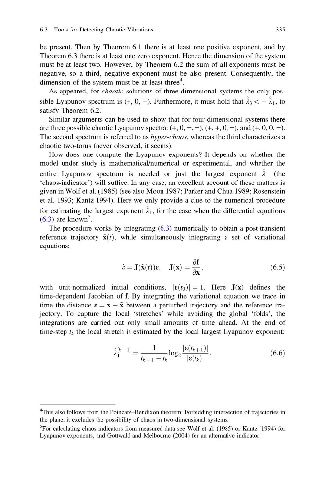
be present. Then by Theorem 6.1 there is at least one positive exponent, and by
Theorem 6.3 there is at least one zero exponent. Hence the dimension of the system
must be at least two. However, by Theorem 6.2 the sum of all exponents must be
negative, so a third, negative exponent must be also present. Consequently, the
dimension of the system must be at least three
4
.
As appeared, for chaotic solutions of three-dimensional systems the only possible Lyapunov spectrum is (+, 0, −). Furthermore, it must hold that ^ k 3 \ À ^ k 1 , to
satisfy Theorem 6.2.
Similar arguments can be used to show that for four-dimensional systems there
are three possible chaotic Lyapunov spectra: (+, 0, −, −), (+, +, 0, −), and (+, 0, 0, −).
The second spectrum is referred to as hyper-chaos, whereas the third characterizes a
chaotic two-torus (never observed, it seems).
How does one compute the Lyapunov exponents? It depends on whether the
model under study is mathematical/numerical or experimental, and whether the
entire Lyapunov spectrum is needed or just the largest exponent ^ k 1 (the
‘chaos-indicator’) will suffice. In any case, an excellent account of these matters is
given in Wolf et al. (1985) (see also Moon 1987; Parker and Chua 1989; Rosenstein
et al. 1993; Kantz 1994). Here we only provide a clue to the numerical procedure
for estimating the largest exponent ^ k 1 , for the case when the differential equations
(6.3) are known
5 .
The procedure works by integrating (6.3) numerically to obtain a post-transient
reference trajectory ~ xðtÞ, while simultaneously integrating a set of variational
equations:
_
e ¼ J ~ xðtÞ
ð
Þe; JðxÞ ¼
@f
@x
;
ð6:5Þ
with unit-normalized initial conditions, eðt 0 Þ
j
j¼ 1. Here J(x) defines the
time-dependent Jacobian of f. By integrating the variational equation we trace in
time the distance e ¼ x À ~ x between a perturbed trajectory and the reference trajectory. To capture the local ‘stretches’ while avoiding the global ‘folds’, the
integrations are carried out only small amounts of time ahead. At the end of
time-step t k the local stretch is estimated by the local largest Lyapunov exponent:
^ k
k þ 1
½
1
¼
1
t k þ 1 À t k
log 2
eðt k þ 1 Þ
j
j
eðt k Þ
j
j
:
ð6:6Þ
4
This also follows from the Poincaré–Bendixon theorem: Forbidding intersection of trajectories in
the plane, it excludes the possibility of chaos in two-dimensional systems.
5
For calculating chaos indicators from measured data see Wolf et al. (1985) or Kantz (1994) for
Lyapunov exponents, and Gottwald and Melbourne (2004) for an alternative indicator.
6.3 Tools for Detecting Chaotic Vibrations
335
Theorem 6.3 there is at least one zero exponent. Hence the dimension of the system
must be at least two. However, by Theorem 6.2 the sum of all exponents must be
negative, so a third, negative exponent must be also present. Consequently, the
dimension of the system must be at least three
4
.
As appeared, for chaotic solutions of three-dimensional systems the only possible Lyapunov spectrum is (+, 0, −). Furthermore, it must hold that ^ k 3 \ À ^ k 1 , to
satisfy Theorem 6.2.
Similar arguments can be used to show that for four-dimensional systems there
are three possible chaotic Lyapunov spectra: (+, 0, −, −), (+, +, 0, −), and (+, 0, 0, −).
The second spectrum is referred to as hyper-chaos, whereas the third characterizes a
chaotic two-torus (never observed, it seems).
How does one compute the Lyapunov exponents? It depends on whether the
model under study is mathematical/numerical or experimental, and whether the
entire Lyapunov spectrum is needed or just the largest exponent ^ k 1 (the
‘chaos-indicator’) will suffice. In any case, an excellent account of these matters is
given in Wolf et al. (1985) (see also Moon 1987; Parker and Chua 1989; Rosenstein
et al. 1993; Kantz 1994). Here we only provide a clue to the numerical procedure
for estimating the largest exponent ^ k 1 , for the case when the differential equations
(6.3) are known
5 .
The procedure works by integrating (6.3) numerically to obtain a post-transient
reference trajectory ~ xðtÞ, while simultaneously integrating a set of variational
equations:
_
e ¼ J ~ xðtÞ
ð
Þe; JðxÞ ¼
@f
@x
;
ð6:5Þ
with unit-normalized initial conditions, eðt 0 Þ
j
j¼ 1. Here J(x) defines the
time-dependent Jacobian of f. By integrating the variational equation we trace in
time the distance e ¼ x À ~ x between a perturbed trajectory and the reference trajectory. To capture the local ‘stretches’ while avoiding the global ‘folds’, the
integrations are carried out only small amounts of time ahead. At the end of
time-step t k the local stretch is estimated by the local largest Lyapunov exponent:
^ k
k þ 1
½
1
¼
1
t k þ 1 À t k
log 2
eðt k þ 1 Þ
j
j
eðt k Þ
j
j
:
ð6:6Þ
4
This also follows from the Poincaré–Bendixon theorem: Forbidding intersection of trajectories in
the plane, it excludes the possibility of chaos in two-dimensional systems.
5
For calculating chaos indicators from measured data see Wolf et al. (1985) or Kantz (1994) for
Lyapunov exponents, and Gottwald and Melbourne (2004) for an alternative indicator.
6.3 Tools for Detecting Chaotic Vibrations
335