

After N time-steps the estimate of the global largest exponent is computed as the
average:
^ k
N
½
1 ¼
1
N
X N
k¼1
k
k
½
1 :
ð6:7Þ
For chaotic attractors the reference trajectory will continue to visit new regions
of phase space, possibly with different local Lyapunov exponents. Estimates of
positive Lyapunov exponents therefore require some time to converge, and a running average estimate may continue to fluctuate. For non-chaotic attractors, i.e.
equilibrium points and limit cycles, the trajectory repeatedly visits the same
localized regions of phase space, giving a much faster rate of convergence for
estimates of negative exponents.
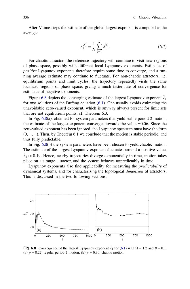
Figure 6.8 depicts the converging estimate of the largest Lyapunov exponent ^ k 1
for two solutions of the Duffing equation (6.1). One usually avoids estimating the
unavoidable zero-valued exponent, which is anyway always present for limit sets
that are not equilibrium points, cf. Theorem 6.3.
In Fig. 6.8(a), obtained for system parameters that yield stable period-2 motion,
the estimate of the largest exponent converges towards the value −0.06. Since the
zero-valued exponent has been ignored, the Lyapunov spectrum must have the form
(0, −, −). Then, by Theorem 6.1 we conclude that the motion is stable periodic, and
thus fully predictable.
In Fig. 6.8(b) the system parameters have been chosen to yield chaotic motion.
The estimate of the largest Lyapunov exponent fluctuates around a positive value,
^ k 1 % 0:19. Hence, nearby trajectories diverge exponentially in time, motion takes
place on a strange attractor, and the system behaves unpredictably in time.
Lyapunov exponents also find applicability for measuring the predictability of
dynamical systems, and for characterizing the topological dimension of attractors;
This is discussed in the two following sections.
Fig. 6.8 Convergence of the largest Lyapunov exponent ^ k 1 for (6.1) with X = 1.2 and b = 0.1.
(a) p = 0.27, regular period-2 motion; (b) p = 0.30, chaotic motion
336
6 Chaotic Vibrations
average:
^ k
N
½
1 ¼
1
N
X N
k¼1
k
k
½
1 :
ð6:7Þ
For chaotic attractors the reference trajectory will continue to visit new regions
of phase space, possibly with different local Lyapunov exponents. Estimates of
positive Lyapunov exponents therefore require some time to converge, and a running average estimate may continue to fluctuate. For non-chaotic attractors, i.e.
equilibrium points and limit cycles, the trajectory repeatedly visits the same
localized regions of phase space, giving a much faster rate of convergence for
estimates of negative exponents.
Figure 6.8 depicts the converging estimate of the largest Lyapunov exponent ^ k 1
for two solutions of the Duffing equation (6.1). One usually avoids estimating the
unavoidable zero-valued exponent, which is anyway always present for limit sets
that are not equilibrium points, cf. Theorem 6.3.
In Fig. 6.8(a), obtained for system parameters that yield stable period-2 motion,
the estimate of the largest exponent converges towards the value −0.06. Since the
zero-valued exponent has been ignored, the Lyapunov spectrum must have the form
(0, −, −). Then, by Theorem 6.1 we conclude that the motion is stable periodic, and
thus fully predictable.
In Fig. 6.8(b) the system parameters have been chosen to yield chaotic motion.
The estimate of the largest Lyapunov exponent fluctuates around a positive value,
^ k 1 % 0:19. Hence, nearby trajectories diverge exponentially in time, motion takes
place on a strange attractor, and the system behaves unpredictably in time.
Lyapunov exponents also find applicability for measuring the predictability of
dynamical systems, and for characterizing the topological dimension of attractors;
This is discussed in the two following sections.
Fig. 6.8 Convergence of the largest Lyapunov exponent ^ k 1 for (6.1) with X = 1.2 and b = 0.1.
(a) p = 0.27, regular period-2 motion; (b) p = 0.30, chaotic motion
336
6 Chaotic Vibrations