

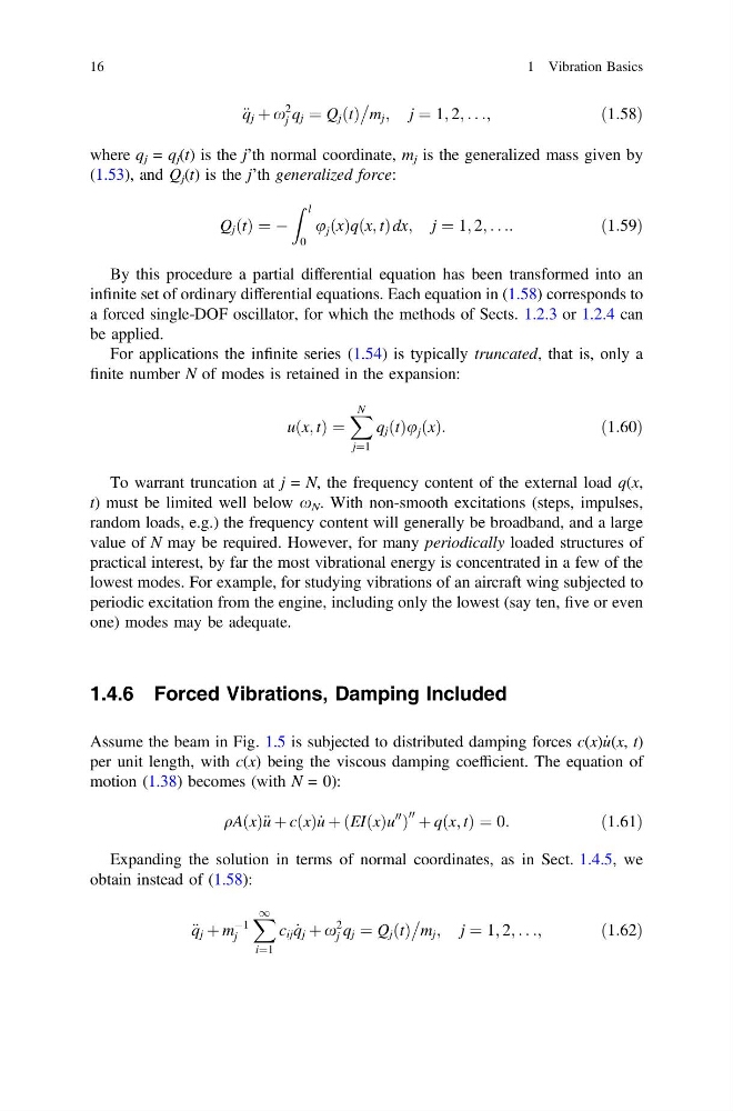
€ q j þ x
2
j q j ¼ Q j ðtÞ
m j ; j ¼ 1; 2; . . .;
ð1:58Þ
where q j = q j (t) is the j’th normal coordinate, m j is the generalized mass given by
(1.53), and Q j (t) is the j’th generalized force:
Q j ðtÞ ¼ À
Z l
0
u j ðxÞqðx; tÞ dx; j ¼ 1; 2; . . .:
ð1:59Þ
By this procedure a partial differential equation has been transformed into an
infinite set of ordinary differential equations. Each equation in (1.58) corresponds to
a forced single-DOF oscillator, for which the methods of Sects. 1.2.3 or 1.2.4 can
be applied.
For applications the infinite series (1.54) is typically truncated, that is, only a
finite number N of modes is retained in the expansion:
uðx; tÞ ¼
X N
j¼1
q j ðtÞu j ðxÞ:
ð1:60Þ
To warrant truncation at j = N, the frequency content of the external load q(x,
t) must be limited well below x N . With non-smooth excitations (steps, impulses,
random loads, e.g.) the frequency content will generally be broadband, and a large
value of N may be required. However, for many periodically loaded structures of
practical interest, by far the most vibrational energy is concentrated in a few of the
lowest modes. For example, for studying vibrations of an aircraft wing subjected to
periodic excitation from the engine, including only the lowest (say ten, five or even
one) modes may be adequate.
1.4.6 Forced Vibrations, Damping Included
Assume the beam in Fig. 1.5 is subjected to distributed damping forces c(x) _
u(x, t)
per unit length, with c(x) being the viscous damping coefficient. The equation of
motion (1.38) becomes (with N = 0):
qAðxÞ€ u þ cðxÞ _
u þ EIðxÞu
00
ð
Þ
00 þ qðx; tÞ ¼ 0:
ð1:61Þ
Expanding the solution in terms of normal coordinates, as in Sect. 1.4.5, we
obtain instead of (1.58):
€ q j þ m
À1
j
X 1
i¼1
c ij _
q j þ x
2
j q j ¼ Q j ðtÞ
m j ; j ¼ 1; 2; . . .;
ð1:62Þ
16
1 Vibration Basics
2
j q j ¼ Q j ðtÞ
m j ; j ¼ 1; 2; . . .;
ð1:58Þ
where q j = q j (t) is the j’th normal coordinate, m j is the generalized mass given by
(1.53), and Q j (t) is the j’th generalized force:
Q j ðtÞ ¼ À
Z l
0
u j ðxÞqðx; tÞ dx; j ¼ 1; 2; . . .:
ð1:59Þ
By this procedure a partial differential equation has been transformed into an
infinite set of ordinary differential equations. Each equation in (1.58) corresponds to
a forced single-DOF oscillator, for which the methods of Sects. 1.2.3 or 1.2.4 can
be applied.
For applications the infinite series (1.54) is typically truncated, that is, only a
finite number N of modes is retained in the expansion:
uðx; tÞ ¼
X N
j¼1
q j ðtÞu j ðxÞ:
ð1:60Þ
To warrant truncation at j = N, the frequency content of the external load q(x,
t) must be limited well below x N . With non-smooth excitations (steps, impulses,
random loads, e.g.) the frequency content will generally be broadband, and a large
value of N may be required. However, for many periodically loaded structures of
practical interest, by far the most vibrational energy is concentrated in a few of the
lowest modes. For example, for studying vibrations of an aircraft wing subjected to
periodic excitation from the engine, including only the lowest (say ten, five or even
one) modes may be adequate.
1.4.6 Forced Vibrations, Damping Included
Assume the beam in Fig. 1.5 is subjected to distributed damping forces c(x) _
u(x, t)
per unit length, with c(x) being the viscous damping coefficient. The equation of
motion (1.38) becomes (with N = 0):
qAðxÞ€ u þ cðxÞ _
u þ EIðxÞu
00
ð
Þ
00 þ qðx; tÞ ¼ 0:
ð1:61Þ
Expanding the solution in terms of normal coordinates, as in Sect. 1.4.5, we
obtain instead of (1.58):
€ q j þ m
À1
j
X 1
i¼1
c ij _
q j þ x
2
j q j ¼ Q j ðtÞ
m j ; j ¼ 1; 2; . . .;
ð1:62Þ
16
1 Vibration Basics