

displaced a small distance q 0 from ~ x t 0
ð Þ. Locally, near t 0 , the distance between the
original and the new solution will grow or shrink as qðtÞ ¼ q 0 2
kðtÀt 0 Þ , that is,
exponentially in time (the base-2 exponential turns out to be more convenient here
than the usual base-e). Imagine now that instead of following just one perturbed
solution, all solutions that start within a tiny ball of radius r(t 0 ) are traced a small
instance of time ahead. The states (x(t), y(t), z(t)) of this bundle of trajectories,
initially within the ball of initial conditions, now evolve within an ellipsoid with
principal axes r j (t), j = 1, 3. The three Lyapunov exponents ^ k 1;2;3 of this system
simply quantify the growth of each of the principal axes, on the average. Suppose,
e.g., that ^ k 1 [ 0 while ^ k 3 \0 ^ k 2 \0. According to (6.4) this implies that one axis of
the ellipsoid is growing while the two others are shrinking. The exponential growth
can be observed only locally, since for real systems the states are bounded so that
escalating orbits sooner or later fold back. Hence, to estimate the Lyapunov
exponents of a solution, one takes the average of many local exponents spread over
the attractor.
As already indicated, a positive Lyapunov exponent implies extreme sensitivity
to initial conditions and thus chaotic motion on a strange attractor. Hence, to detect
whether an observed post-transient motion is chaotic or regular, we merely need to
compute the largest exponent ^ k 1 .
However, given the full spectrum of Lyapunov exponents ^ k j; j ¼ 1; n; ordered as
a sequence ^ k 1 ! ^ k 2 ! . . . ! ^ k n ; it is possible to give a more precise account of the
attractor involved (e.g., Parker and Chua 1989):
Theorem 6.1 Type of attractor in dependency of Lyapunov exponents ^ k j :
Stable equilibrium: ^ k j \0 for j = 1,n
Stable limit cycle: ^ k 1 ¼ 0 and ^ k j \0 for j = 2, n
Stable two-torus:
^ k 1 ¼ ^ k 2 ¼ 0 and ^ k j \0 for j = 3, n
Stable K-torus:
^ k 1 ¼ Á Á Á ¼ ^ k K ¼ 0 and ^ k j \0 for j ¼ K þ 1; n
Chaotic:
^ k 1 [ 0
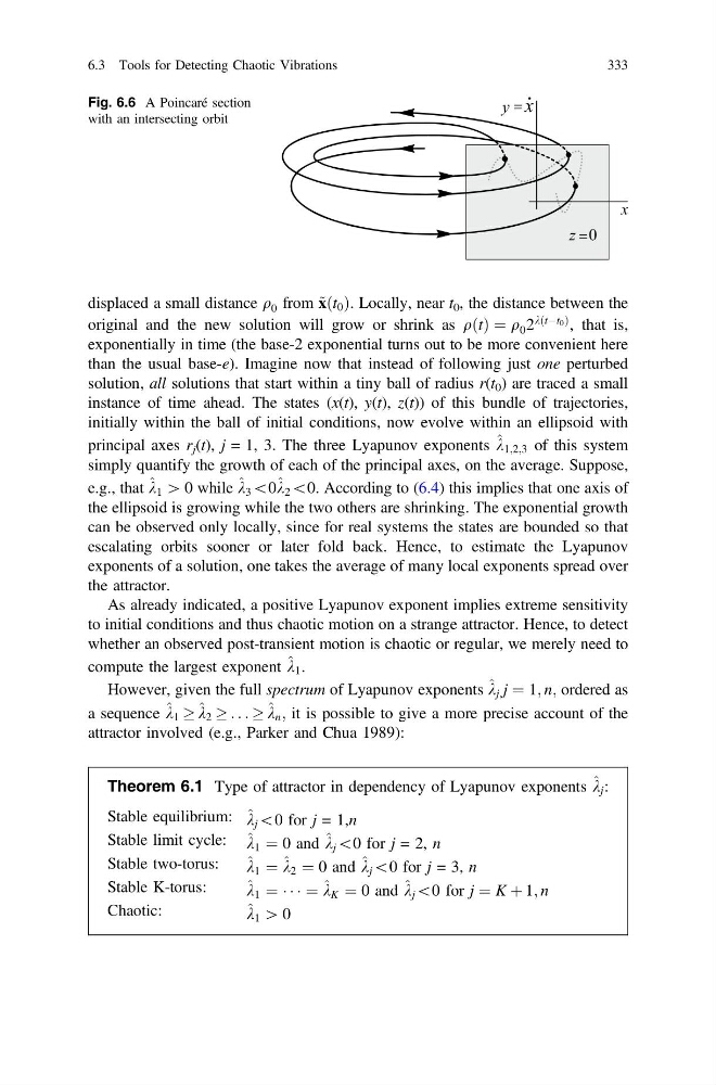
Fig. 6.6 A Poincaré section
with an intersecting orbit
6.3 Tools for Detecting Chaotic Vibrations
333
ð Þ. Locally, near t 0 , the distance between the
original and the new solution will grow or shrink as qðtÞ ¼ q 0 2
kðtÀt 0 Þ , that is,
exponentially in time (the base-2 exponential turns out to be more convenient here
than the usual base-e). Imagine now that instead of following just one perturbed
solution, all solutions that start within a tiny ball of radius r(t 0 ) are traced a small
instance of time ahead. The states (x(t), y(t), z(t)) of this bundle of trajectories,
initially within the ball of initial conditions, now evolve within an ellipsoid with
principal axes r j (t), j = 1, 3. The three Lyapunov exponents ^ k 1;2;3 of this system
simply quantify the growth of each of the principal axes, on the average. Suppose,
e.g., that ^ k 1 [ 0 while ^ k 3 \0 ^ k 2 \0. According to (6.4) this implies that one axis of
the ellipsoid is growing while the two others are shrinking. The exponential growth
can be observed only locally, since for real systems the states are bounded so that
escalating orbits sooner or later fold back. Hence, to estimate the Lyapunov
exponents of a solution, one takes the average of many local exponents spread over
the attractor.
As already indicated, a positive Lyapunov exponent implies extreme sensitivity
to initial conditions and thus chaotic motion on a strange attractor. Hence, to detect
whether an observed post-transient motion is chaotic or regular, we merely need to
compute the largest exponent ^ k 1 .
However, given the full spectrum of Lyapunov exponents ^ k j; j ¼ 1; n; ordered as
a sequence ^ k 1 ! ^ k 2 ! . . . ! ^ k n ; it is possible to give a more precise account of the
attractor involved (e.g., Parker and Chua 1989):
Theorem 6.1 Type of attractor in dependency of Lyapunov exponents ^ k j :
Stable equilibrium: ^ k j \0 for j = 1,n
Stable limit cycle: ^ k 1 ¼ 0 and ^ k j \0 for j = 2, n
Stable two-torus:
^ k 1 ¼ ^ k 2 ¼ 0 and ^ k j \0 for j = 3, n
Stable K-torus:
^ k 1 ¼ Á Á Á ¼ ^ k K ¼ 0 and ^ k j \0 for j ¼ K þ 1; n
Chaotic:
^ k 1 [ 0
Fig. 6.6 A Poincaré section
with an intersecting orbit
6.3 Tools for Detecting Chaotic Vibrations
333