

Experimental Poincaré maps can be obtained by using the external trigger
facility present at most signal analyzers and oscilloscopes. For example, using the
XY-ports of a storage oscilloscope to display the phase plane of a periodically
driven system, one can usually set up an external triggering that intensifies the light
beam at a particular phase of the driving force.
Summing up the possible limit sets of Poincaré maps, we find that a finite
number of points correspond to periodic motion, an infinite number of points filling
up a closed curve corresponds to quasiperiodic motion, and an infinite number of
orderly distributed points (usually) corresponds to chaotic motion.
6.3.4 Lyapunov Exponents
Lyapunov exponents essentially measure the average rates of convergence or
divergence of nearby orbits in phase space. A positive Lyapunov exponent indicates
exponential separation of nearby orbits – a ‘stretching’ of phase space. Since for
real systems the phase space is always bounded this separation cannot go on
forever; Sooner or later orbits have to fold back towards the center of the phase
space. This process of repeated stretching and folding is what characterizes chaos.
Thus, a positive Lyapunov exponent, properly computed, is among the strongest
indicators of chaotic motion.
Consider a general continuous system, written as a set of n autonomous
first-order equations:
_
x ¼ fðxÞ; x ¼ xðtÞ 2 R
n
:
ð6:3Þ
Start the system, by applying some initial conditions, and allow sufficient time
for the system to reach an attractor (that is, cut off transients; cf. e.g. Table 1.4 in
Sect. 1.7.5). The attractor can be an equilibrium point, a limit cycle or a strange
attractor. Now, when the system appears to be on the attractor, define a new time
zero. Record x(0), and consider the solution from thereon ~ x t
ð Þ; t [ 0. To this
particular solution, moving on the particular attractor, we assign exactly
n Lyapunov exponents ^ k j ; j ¼ 1; n. The set of Lyapunov exponents is defined as
follows (Wolf et al. 1985):
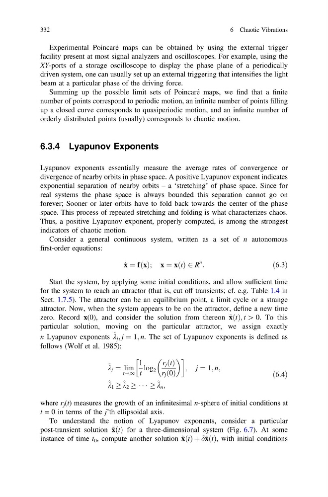
^ k j ¼ lim
t!1
1
t
log 2
r j ðtÞ
r j ð0Þ
!
; j ¼ 1; n;
^ k 1 ! ^ k 2 ! Á Á Á ! ^ k n ;
ð6:4Þ
where r j (t) measures the growth of an infinitesimal n-sphere of initial conditions at
t = 0 in terms of the j’th ellipsoidal axis.
To understand the notion of Lyapunov exponents, consider a particular
post-transient solution ~ x t
ð Þ for a three-dimensional system (Fig. 6.7). At some
instance of time t 0 , compute another solution ~ xðtÞ þ d~ xðtÞ, with initial conditions
332
6 Chaotic Vibrations
facility present at most signal analyzers and oscilloscopes. For example, using the
XY-ports of a storage oscilloscope to display the phase plane of a periodically
driven system, one can usually set up an external triggering that intensifies the light
beam at a particular phase of the driving force.
Summing up the possible limit sets of Poincaré maps, we find that a finite
number of points correspond to periodic motion, an infinite number of points filling
up a closed curve corresponds to quasiperiodic motion, and an infinite number of
orderly distributed points (usually) corresponds to chaotic motion.
6.3.4 Lyapunov Exponents
Lyapunov exponents essentially measure the average rates of convergence or
divergence of nearby orbits in phase space. A positive Lyapunov exponent indicates
exponential separation of nearby orbits – a ‘stretching’ of phase space. Since for
real systems the phase space is always bounded this separation cannot go on
forever; Sooner or later orbits have to fold back towards the center of the phase
space. This process of repeated stretching and folding is what characterizes chaos.
Thus, a positive Lyapunov exponent, properly computed, is among the strongest
indicators of chaotic motion.
Consider a general continuous system, written as a set of n autonomous
first-order equations:
_
x ¼ fðxÞ; x ¼ xðtÞ 2 R
n
:
ð6:3Þ
Start the system, by applying some initial conditions, and allow sufficient time
for the system to reach an attractor (that is, cut off transients; cf. e.g. Table 1.4 in
Sect. 1.7.5). The attractor can be an equilibrium point, a limit cycle or a strange
attractor. Now, when the system appears to be on the attractor, define a new time
zero. Record x(0), and consider the solution from thereon ~ x t
ð Þ; t [ 0. To this
particular solution, moving on the particular attractor, we assign exactly
n Lyapunov exponents ^ k j ; j ¼ 1; n. The set of Lyapunov exponents is defined as
follows (Wolf et al. 1985):
^ k j ¼ lim
t!1
1
t
log 2
r j ðtÞ
r j ð0Þ
!
; j ¼ 1; n;
^ k 1 ! ^ k 2 ! Á Á Á ! ^ k n ;
ð6:4Þ
where r j (t) measures the growth of an infinitesimal n-sphere of initial conditions at
t = 0 in terms of the j’th ellipsoidal axis.
To understand the notion of Lyapunov exponents, consider a particular
post-transient solution ~ x t
ð Þ for a three-dimensional system (Fig. 6.7). At some
instance of time t 0 , compute another solution ~ xðtÞ þ d~ xðtÞ, with initial conditions
332
6 Chaotic Vibrations