

plot _
x(t) versus x(t). This plot traces out a continuous curve in the phase plane.
Considering instead the values of the two state variables _
x and x only at discrete
times t k , k = 0, 1, 2, …, the motion will appear as a sequence of dots in the phase
plane. The continuous flow of states becomes replaced by a two-dimensional map,
mapping states at time t k on states at a later time t k+1 . Choosing the time instances t k
according to certain rules, the map will be a Poincaré map.
For systems subjected to external periodic forcing the Poincaré map is usually
obtained by choosing t k = t 0 + kT, k = 0, 1, 2, …, where T is the period of the
driving force. Thus for (6.1) we plot the sequence of points (x(t k ),_ x(t k )) with t k =
t 0 + k2p/X. This is very much like observing the phase plane motion using a
stroboscope that flashes at a particular phase Xt 0 of the driving force, recording only
the ‘flash’-values of (x(t),_ x(t)).
Fig. 6.5(a) shows a Poincaré map for (6.1) obtained with t 0 = 0. It corresponds
to a sampling of the phase plot in Fig. 6.3(a) at times t k = k2p/X. The map consists
of a finite number of points, implying periodic motion. In fact, there are two points,
indicating period-2 motion. Period-n motion generally shows up as n points in the
Poincaré map, whereas quasiperiodic motion reveals itself as infinitely many points
filling up a closed curve.
Fig. 6.5(b) shows a Poincaré map similarly obtained, corresponding to the
chaotic phase-plane orbit of Fig. 6.3(b). As simulation time marches on, more and
more points will be added to the map. However, they will continue to do so in an
orderly manner, filling out details of the strange creature you see in the figure.
Indeed, what the figure shows is a two-dimensional cross-section of a so-called
strange attractor on which the chaotic motion rides. We shall return to the
‘strangeness’ of strange attractors, which turns out to be associated with a
non-integer topological dimension. Suffice here to say that a post-transient Poincaré
map that consists neither of a finite number of points, nor of points filling up a
closed curve, but nevertheless appears ordered – is a strong indicator of deterministic chaos. For some chaotic systems the Poincaré points will spread all over
the map. This kind of behavior, known as Hamiltonian chaos, is typically found
when there is no or very little dissipation in the system.
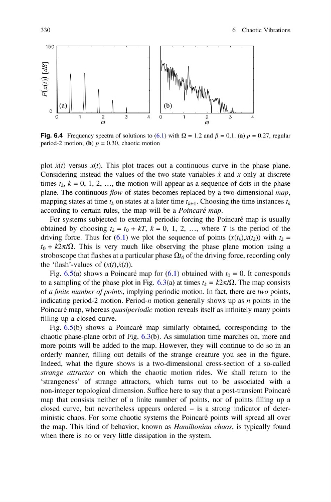
Fig. 6.4 Frequency spectra of solutions to (6.1) with X = 1.2 and b = 0.1. (a) p = 0.27, regular
period-2 motion; (b) p = 0.30, chaotic motion
330
6 Chaotic Vibrations
x(t) versus x(t). This plot traces out a continuous curve in the phase plane.
Considering instead the values of the two state variables _
x and x only at discrete
times t k , k = 0, 1, 2, …, the motion will appear as a sequence of dots in the phase
plane. The continuous flow of states becomes replaced by a two-dimensional map,
mapping states at time t k on states at a later time t k+1 . Choosing the time instances t k
according to certain rules, the map will be a Poincaré map.
For systems subjected to external periodic forcing the Poincaré map is usually
obtained by choosing t k = t 0 + kT, k = 0, 1, 2, …, where T is the period of the
driving force. Thus for (6.1) we plot the sequence of points (x(t k ),_ x(t k )) with t k =
t 0 + k2p/X. This is very much like observing the phase plane motion using a
stroboscope that flashes at a particular phase Xt 0 of the driving force, recording only
the ‘flash’-values of (x(t),_ x(t)).
Fig. 6.5(a) shows a Poincaré map for (6.1) obtained with t 0 = 0. It corresponds
to a sampling of the phase plot in Fig. 6.3(a) at times t k = k2p/X. The map consists
of a finite number of points, implying periodic motion. In fact, there are two points,
indicating period-2 motion. Period-n motion generally shows up as n points in the
Poincaré map, whereas quasiperiodic motion reveals itself as infinitely many points
filling up a closed curve.
Fig. 6.5(b) shows a Poincaré map similarly obtained, corresponding to the
chaotic phase-plane orbit of Fig. 6.3(b). As simulation time marches on, more and
more points will be added to the map. However, they will continue to do so in an
orderly manner, filling out details of the strange creature you see in the figure.
Indeed, what the figure shows is a two-dimensional cross-section of a so-called
strange attractor on which the chaotic motion rides. We shall return to the
‘strangeness’ of strange attractors, which turns out to be associated with a
non-integer topological dimension. Suffice here to say that a post-transient Poincaré
map that consists neither of a finite number of points, nor of points filling up a
closed curve, but nevertheless appears ordered – is a strong indicator of deterministic chaos. For some chaotic systems the Poincaré points will spread all over
the map. This kind of behavior, known as Hamiltonian chaos, is typically found
when there is no or very little dissipation in the system.
Fig. 6.4 Frequency spectra of solutions to (6.1) with X = 1.2 and b = 0.1. (a) p = 0.27, regular
period-2 motion; (b) p = 0.30, chaotic motion
330
6 Chaotic Vibrations