

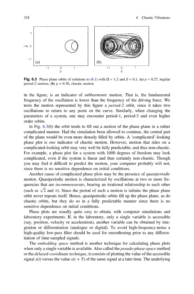
in the figure, is an indicator of subharmonic motion. That is, the fundamental
frequency of the oscillation is lower than the frequency of the driving force. We
term the motion represented by this figure a period-2 orbit, since it takes two
oscillations to return to any point on the curve. Similarly, when changing the
parameters of a system, one may encounter period-1, period-3 and even higher
order orbits.
In Fig. 6.3(b) the orbit tends to fill out a section of the phase plane in a rather
complicated manner. Had the simulation been allowed to continue, the central part
of the plane would be even more densely filled by orbits. A ‘complicated’-looking
phase plot is one indicator of chaotic motion. However, motion that rides on a
complicated-looking orbit may very well be fully predictable, and thus non-chaotic.
For example, a phase plot for a system with 1000 degrees of freedom may look
complicated, even if the system is linear and thus certainly non-chaotic. Though
you may find it difficult to predict the motion, your computer probably will not,
since there is no sensitive dependence on initial conditions.
Another cause of complicated phase plots may be the presence of quasiperiodic
motion. Quasiperiodic motion is characterized by oscillations at two or more frequencies that are incommensurate, bearing an irrational relationship to each other
(such as
ffiffi ffi
2
p
and p). Since the period of such a motion is infinite the phase plane
orbit never repeats itself. Hence, quasiperiodic orbits fill up the phase plane, as do
chaotic orbits, but they do so in a fully predictable manner since there is no
sensitive dependence on initial conditions.
Phase plots are usually quite easy to obtain, with computer simulations and
laboratory experiments. If, in the laboratory, only a single variable is accessible
(say, position, velocity or acceleration), another variable can be obtained by integration or differentiation (analogue or digital). To avoid high-frequency-noise a
high-quality low-pass filter should be used for smoothening prior to any differentiation of time-sampled signals.
The embedding space method is another technique for calculating phase plots
when only a single variable is available. Also called the pseudo-phase-space method
or the delayed-coordinate technique, it consists of plotting the value of the accessible
signal x(t) versus the value x(t + T) of the same signal at a later time. The underlying
Fig. 6.3 Phase plane orbits of solutions to (6.1) with X = 1.2 and b = 0.1. (a) p = 0.27, regular
period-2 motion; (b) p = 0.30, chaotic motion
328
6 Chaotic Vibrations
frequency of the oscillation is lower than the frequency of the driving force. We
term the motion represented by this figure a period-2 orbit, since it takes two
oscillations to return to any point on the curve. Similarly, when changing the
parameters of a system, one may encounter period-1, period-3 and even higher
order orbits.
In Fig. 6.3(b) the orbit tends to fill out a section of the phase plane in a rather
complicated manner. Had the simulation been allowed to continue, the central part
of the plane would be even more densely filled by orbits. A ‘complicated’-looking
phase plot is one indicator of chaotic motion. However, motion that rides on a
complicated-looking orbit may very well be fully predictable, and thus non-chaotic.
For example, a phase plot for a system with 1000 degrees of freedom may look
complicated, even if the system is linear and thus certainly non-chaotic. Though
you may find it difficult to predict the motion, your computer probably will not,
since there is no sensitive dependence on initial conditions.
Another cause of complicated phase plots may be the presence of quasiperiodic
motion. Quasiperiodic motion is characterized by oscillations at two or more frequencies that are incommensurate, bearing an irrational relationship to each other
(such as
ffiffi ffi
2
p
and p). Since the period of such a motion is infinite the phase plane
orbit never repeats itself. Hence, quasiperiodic orbits fill up the phase plane, as do
chaotic orbits, but they do so in a fully predictable manner since there is no
sensitive dependence on initial conditions.
Phase plots are usually quite easy to obtain, with computer simulations and
laboratory experiments. If, in the laboratory, only a single variable is accessible
(say, position, velocity or acceleration), another variable can be obtained by integration or differentiation (analogue or digital). To avoid high-frequency-noise a
high-quality low-pass filter should be used for smoothening prior to any differentiation of time-sampled signals.
The embedding space method is another technique for calculating phase plots
when only a single variable is available. Also called the pseudo-phase-space method
or the delayed-coordinate technique, it consists of plotting the value of the accessible
signal x(t) versus the value x(t + T) of the same signal at a later time. The underlying
Fig. 6.3 Phase plane orbits of solutions to (6.1) with X = 1.2 and b = 0.1. (a) p = 0.27, regular
period-2 motion; (b) p = 0.30, chaotic motion
328
6 Chaotic Vibrations