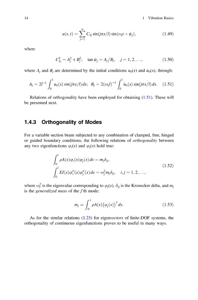
uðx; tÞ ¼
X 1
j¼1
C 1j sinðjpx=lÞ sinðx j t þ w j Þ;
ð1:49Þ
where
C
2
1j ¼ A
2
j þ B
2
j ; tan w j ¼ A j
B j ; j ¼ 1; 2; . . .;
ð1:50Þ
where A j and B j are determined by the initial conditions u 0 (x) and _
u 0 (x), through:
A j ¼ 2l
À1
Z l
0
u 0 ðxÞ sinðjpx=lÞ dx; B j ¼ 2ðx j lÞ
À1
Z l
0
_
u 0 ðxÞ sinðjpx=lÞ dx: ð1:51Þ
Relations of orthogonality have been employed for obtaining (1.51). These will
be presented next.
1.4.3 Orthogonality of Modes
For a variable section beam subjected to any combination of clamped, free, hinged
or guided boundary conditions, the following relations of orthogonality between
any two eigenfunctions u i (x) and u j (x) hold true:
Z l
0
qAðxÞu i ðxÞu j ðxÞ dx ¼ m j d ij ;
Z l
0
EIðxÞu
00
i ðxÞu
00
j ðxÞdx ¼ x
2
j m j d ij ; i; j ¼ 1; 2; . . .;
ð1:52Þ
where x j
2 is the eigenvalue corresponding to u j (x), d ij is the Kronecker delta, and m j
is the generalized mass of the j’th mode:
m j ¼
Z l
0
qAðxÞ u j ðxÞ
À
Á 2 dx:
ð1:53Þ
As for the similar relations (1.23) for eigenvectors of finite-DOF systems, the
orthogonality of continuous eigenfunctions proves to be useful in many ways.
14
1 Vibration Basics