

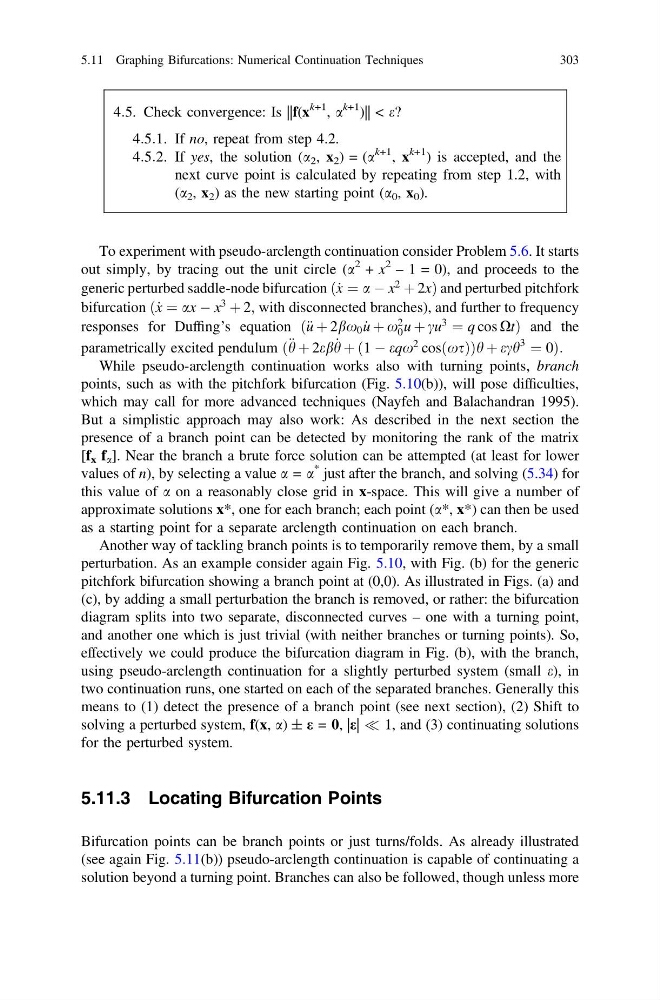
4:5. Check convergence: Is ||f(x
k+1 , a
k+1 )|| < e?
4:5:1. If no, repeat from step 4.2.
4:5:2. If yes, the solution (a 2 , x 2 ) = (a
k+1 , x
k+1 ) is accepted, and the
next curve point is calculated by repeating from step 1.2, with
(a 2 , x 2 ) as the new starting point (a 0 , x 0 ).
To experiment with pseudo-arclength continuation consider Problem 5.6. It starts
out simply, by tracing out the unit circle (a
2 + x
2
– 1 = 0), and proceeds to the
generic perturbed saddle-node bifurcation ð_ x ¼ a À x
2
þ 2xÞ and perturbed pitchfork
bifurcation ð_ x ¼ ax À x
3
þ 2; with disconnected branches), and further to frequency
responses for Duffing’s equation ð€ u þ 2bx 0 _
u þ x
2
0 u þ cu
3
¼ q cos XtÞ and the
parametrically excited pendulum ð € h þ 2eb _
h þ ð1 À eqx
2 cosðxsÞÞh þ ech
3
¼ 0Þ:
While pseudo-arclength continuation works also with turning points, branch
points, such as with the pitchfork bifurcation (Fig. 5.10(b)), will pose difficulties,
which may call for more advanced techniques (Nayfeh and Balachandran 1995).
But a simplistic approach may also work: As described in the next section the
presence of a branch point can be detected by monitoring the rank of the matrix
[f x f a ]. Near the branch a brute force solution can be attempted (at least for lower
values of n), by selecting a value a = a
* just after the branch, and solving (5.34) for
this value of a on a reasonably close grid in x-space. This will give a number of
approximate solutions x*, one for each branch; each point (a*, x*) can then be used
as a starting point for a separate arclength continuation on each branch.
Another way of tackling branch points is to temporarily remove them, by a small
perturbation. As an example consider again Fig. 5.10, with Fig. (b) for the generic
pitchfork bifurcation showing a branch point at (0,0). As illustrated in Figs. (a) and
(c), by adding a small perturbation the branch is removed, or rather: the bifurcation
diagram splits into two separate, disconnected curves – one with a turning point,
and another one which is just trivial (with neither branches or turning points). So,
effectively we could produce the bifurcation diagram in Fig. (b), with the branch,
using pseudo-arclength continuation for a slightly perturbed system (small e), in
two continuation runs, one started on each of the separated branches. Generally this
means to (1) detect the presence of a branch point (see next section), (2) Shift to
solving a perturbed system, f(x, a) ± e = 0, |e| ( 1, and (3) continuating solutions
for the perturbed system.
5.11.3 Locating Bifurcation Points
Bifurcation points can be branch points or just turns/folds. As already illustrated
(see again Fig. 5.11(b)) pseudo-arclength continuation is capable of continuating a
solution beyond a turning point. Branches can also be followed, though unless more
5.11 Graphing Bifurcations: Numerical Continuation Techniques
303
k+1 , a
k+1 )|| < e?
4:5:1. If no, repeat from step 4.2.
4:5:2. If yes, the solution (a 2 , x 2 ) = (a
k+1 , x
k+1 ) is accepted, and the
next curve point is calculated by repeating from step 1.2, with
(a 2 , x 2 ) as the new starting point (a 0 , x 0 ).
To experiment with pseudo-arclength continuation consider Problem 5.6. It starts
out simply, by tracing out the unit circle (a
2 + x
2
– 1 = 0), and proceeds to the
generic perturbed saddle-node bifurcation ð_ x ¼ a À x
2
þ 2xÞ and perturbed pitchfork
bifurcation ð_ x ¼ ax À x
3
þ 2; with disconnected branches), and further to frequency
responses for Duffing’s equation ð€ u þ 2bx 0 _
u þ x
2
0 u þ cu
3
¼ q cos XtÞ and the
parametrically excited pendulum ð € h þ 2eb _
h þ ð1 À eqx
2 cosðxsÞÞh þ ech
3
¼ 0Þ:
While pseudo-arclength continuation works also with turning points, branch
points, such as with the pitchfork bifurcation (Fig. 5.10(b)), will pose difficulties,
which may call for more advanced techniques (Nayfeh and Balachandran 1995).
But a simplistic approach may also work: As described in the next section the
presence of a branch point can be detected by monitoring the rank of the matrix
[f x f a ]. Near the branch a brute force solution can be attempted (at least for lower
values of n), by selecting a value a = a
* just after the branch, and solving (5.34) for
this value of a on a reasonably close grid in x-space. This will give a number of
approximate solutions x*, one for each branch; each point (a*, x*) can then be used
as a starting point for a separate arclength continuation on each branch.
Another way of tackling branch points is to temporarily remove them, by a small
perturbation. As an example consider again Fig. 5.10, with Fig. (b) for the generic
pitchfork bifurcation showing a branch point at (0,0). As illustrated in Figs. (a) and
(c), by adding a small perturbation the branch is removed, or rather: the bifurcation
diagram splits into two separate, disconnected curves – one with a turning point,
and another one which is just trivial (with neither branches or turning points). So,
effectively we could produce the bifurcation diagram in Fig. (b), with the branch,
using pseudo-arclength continuation for a slightly perturbed system (small e), in
two continuation runs, one started on each of the separated branches. Generally this
means to (1) detect the presence of a branch point (see next section), (2) Shift to
solving a perturbed system, f(x, a) ± e = 0, |e| ( 1, and (3) continuating solutions
for the perturbed system.
5.11.3 Locating Bifurcation Points
Bifurcation points can be branch points or just turns/folds. As already illustrated
(see again Fig. 5.11(b)) pseudo-arclength continuation is capable of continuating a
solution beyond a turning point. Branches can also be followed, though unless more
5.11 Graphing Bifurcations: Numerical Continuation Techniques
303