

sophisticated algorithms are used, initial starting points needs to be located on each
branch. But how do we locate the bifurcation points? Due to the finite stepsize Ds,
the pseudo-arclength algorithm is unlikely to end up exactly at the turning or branch
point; in fact that would make the algorithm fail, since the Jacobian f x is singular at
the turning point so that (5.42) is unsolvable.
However, the singularity of f x at turning and branch points can be used to locate
bifurcation points, e.g. by monitoring |f x |, or the rank or eigenvalues of f x versus the
parameter a or s. As a static bifurcation point is approached, one of the eigenvalues
of f x will approach zero (and the rank of f x will decrease to n − 1). As a Hopf
bifurcation is approached, the eigenvalues of f x will approach a purely imaginary
pair ±ix, with all other eigenvalues having nonzero real parts.
Furthermore, the rank of the extended matrix [f x f a ] (i.e. the coefficient matrix of
the homogeneous system (5.38) for determining the tangent vector) can be used to
determine if the bifurcation is a turning or a branch point: [f x f a ] has rank n at
saddle-node bifurcations, but rank n − 1 at other static bifurcation points (Nayfeh
and Balachandran 1995). This reflects that saddle-node bifurcations have
well-defined and continuously changing tangents (t in (5.38)), while this is not so
for the other static bifurcations; the pitchfork and the transcritical bifurcations, with
their branches, have no well-defined tangent. So: f = 0 with rank(f x ) = n − 1 marks
a bifurcation; this bifurcation is of the turning point type if rank([f x f a ]) = n, while
of the branching type if rank([f x f a ]) = n − 1.
The bifurcation detection methods described in this section are called indirect;
they do not imply systematic search for bifurcation points, but are based just on
monitoring properties of quantities that are anyway calculated during the continuation process. Direct methods, by contrast, relies on systematically searching for
bifurcation points, e.g. by setting up equations that have bifurcation points as
solutions. For example, at a bifurcation point (x, a) must satisfy:
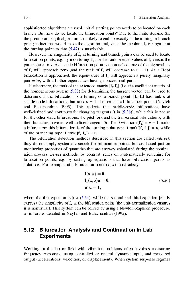
fðx; aÞ ¼ 0;
f x ðx; aÞu ¼ 0;
u
T
u ¼ 1;
ð5:50Þ
where the first equation is just (5.34), while the second and third equation jointly
express the singularity of f x at the bifurcation point (the unit-normalization ensures
u is nontrivial). This system can be solved by using a Newton-Raphson procedure,
as is further detailed in Nayfeh and Balachandran (1995).
5.12 Bifurcation Analysis and Continuation in Lab
Experiments
Working in the lab or field with vibration problems often involves measuring
frequency responses, using controlled or natural dynamic input, and measured
output (accelerations, velocities, or displacement). When system response regimes
304
5 Bifurcation Analysis
branch. But how do we locate the bifurcation points? Due to the finite stepsize Ds,
the pseudo-arclength algorithm is unlikely to end up exactly at the turning or branch
point; in fact that would make the algorithm fail, since the Jacobian f x is singular at
the turning point so that (5.42) is unsolvable.
However, the singularity of f x at turning and branch points can be used to locate
bifurcation points, e.g. by monitoring |f x |, or the rank or eigenvalues of f x versus the
parameter a or s. As a static bifurcation point is approached, one of the eigenvalues
of f x will approach zero (and the rank of f x will decrease to n − 1). As a Hopf
bifurcation is approached, the eigenvalues of f x will approach a purely imaginary
pair ±ix, with all other eigenvalues having nonzero real parts.
Furthermore, the rank of the extended matrix [f x f a ] (i.e. the coefficient matrix of
the homogeneous system (5.38) for determining the tangent vector) can be used to
determine if the bifurcation is a turning or a branch point: [f x f a ] has rank n at
saddle-node bifurcations, but rank n − 1 at other static bifurcation points (Nayfeh
and Balachandran 1995). This reflects that saddle-node bifurcations have
well-defined and continuously changing tangents (t in (5.38)), while this is not so
for the other static bifurcations; the pitchfork and the transcritical bifurcations, with
their branches, have no well-defined tangent. So: f = 0 with rank(f x ) = n − 1 marks
a bifurcation; this bifurcation is of the turning point type if rank([f x f a ]) = n, while
of the branching type if rank([f x f a ]) = n − 1.
The bifurcation detection methods described in this section are called indirect;
they do not imply systematic search for bifurcation points, but are based just on
monitoring properties of quantities that are anyway calculated during the continuation process. Direct methods, by contrast, relies on systematically searching for
bifurcation points, e.g. by setting up equations that have bifurcation points as
solutions. For example, at a bifurcation point (x, a) must satisfy:
fðx; aÞ ¼ 0;
f x ðx; aÞu ¼ 0;
u
T
u ¼ 1;
ð5:50Þ
where the first equation is just (5.34), while the second and third equation jointly
express the singularity of f x at the bifurcation point (the unit-normalization ensures
u is nontrivial). This system can be solved by using a Newton-Raphson procedure,
as is further detailed in Nayfeh and Balachandran (1995).
5.12 Bifurcation Analysis and Continuation in Lab
Experiments
Working in the lab or field with vibration problems often involves measuring
frequency responses, using controlled or natural dynamic input, and measured
output (accelerations, velocities, or displacement). When system response regimes
304
5 Bifurcation Analysis