

€ u þ _
u À ku þ u
2
¼ 0;
ð5:22Þ
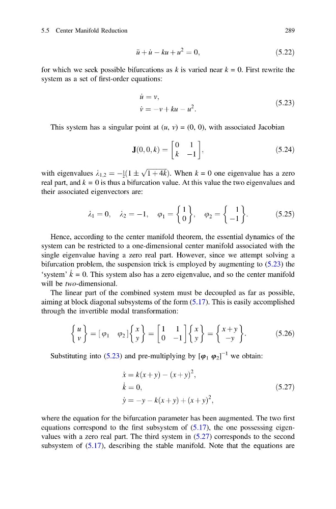
for which we seek possible bifurcations as k is varied near k = 0. First rewrite the
system as a set of first-order equations:
_
u ¼ v;
_
v ¼ Àv þ ku À u
2
:
ð5:23Þ
This system has a singular point at (u, v) = (0, 0), with associated Jacobian
Jð0; 0; kÞ ¼
0 1
k À1
!
;
ð5:24Þ
with eigenvalues k 1;2 ¼ À
1
2 ð1 Æ
ffiffiffiffiffiffiffiffiffiffiffiffi ffi
1 þ 4k
p
Þ. When k = 0 one eigenvalue has a zero
real part, and k = 0 is thus a bifurcation value. At this value the two eigenvalues and
their associated eigenvectors are:
k 1 ¼ 0; k 2 ¼ À1; u 1 ¼
1
0
& '
; u 2 ¼
1
À1
&
'
:
ð5:25Þ
Hence, according to the center manifold theorem, the essential dynamics of the
system can be restricted to a one-dimensional center manifold associated with the
single eigenvalue having a zero real part. However, since we attempt solving a
bifurcation problem, the suspension trick is employed by augmenting to (5.23) the
‘system’ _
k = 0. This system also has a zero eigenvalue, and so the center manifold
will be two-dimensional.
The linear part of the combined system must be decoupled as far as possible,
aiming at block diagonal subsystems of the form (5.17). This is easily accomplished
through the invertible modal transformation:
u
v
& '
¼ u 1 u 2
½
x
y
& '
¼
1 1
0 À1
!
x
y
& '
¼
x þ y
Ày
&
'
:
ð5:26Þ
Substituting into (5.23) and pre-multiplying by [u 1 u 2 ]
−1 we obtain:
_
x ¼ kðx þ yÞ À ðx þ yÞ
2 ;
_
k ¼ 0;
_
y ¼ Ày À kðx þ yÞ þ ðx þ yÞ
2 ;
ð5:27Þ
where the equation for the bifurcation parameter has been augmented. The two first
equations correspond to the first subsystem of (5.17), the one possessing eigenvalues with a zero real part. The third system in (5.27) corresponds to the second
subsystem of (5.17), describing the stable manifold. Note that the equations are
5.5 Center Manifold Reduction
289
u À ku þ u
2
¼ 0;
ð5:22Þ
for which we seek possible bifurcations as k is varied near k = 0. First rewrite the
system as a set of first-order equations:
_
u ¼ v;
_
v ¼ Àv þ ku À u
2
:
ð5:23Þ
This system has a singular point at (u, v) = (0, 0), with associated Jacobian
Jð0; 0; kÞ ¼
0 1
k À1
!
;
ð5:24Þ
with eigenvalues k 1;2 ¼ À
1
2 ð1 Æ
ffiffiffiffiffiffiffiffiffiffiffiffi ffi
1 þ 4k
p
Þ. When k = 0 one eigenvalue has a zero
real part, and k = 0 is thus a bifurcation value. At this value the two eigenvalues and
their associated eigenvectors are:
k 1 ¼ 0; k 2 ¼ À1; u 1 ¼
1
0
& '
; u 2 ¼
1
À1
&
'
:
ð5:25Þ
Hence, according to the center manifold theorem, the essential dynamics of the
system can be restricted to a one-dimensional center manifold associated with the
single eigenvalue having a zero real part. However, since we attempt solving a
bifurcation problem, the suspension trick is employed by augmenting to (5.23) the
‘system’ _
k = 0. This system also has a zero eigenvalue, and so the center manifold
will be two-dimensional.
The linear part of the combined system must be decoupled as far as possible,
aiming at block diagonal subsystems of the form (5.17). This is easily accomplished
through the invertible modal transformation:
u
v
& '
¼ u 1 u 2
½
x
y
& '
¼
1 1
0 À1
!
x
y
& '
¼
x þ y
Ày
&
'
:
ð5:26Þ
Substituting into (5.23) and pre-multiplying by [u 1 u 2 ]
−1 we obtain:
_
x ¼ kðx þ yÞ À ðx þ yÞ
2 ;
_
k ¼ 0;
_
y ¼ Ày À kðx þ yÞ þ ðx þ yÞ
2 ;
ð5:27Þ
where the equation for the bifurcation parameter has been augmented. The two first
equations correspond to the first subsystem of (5.17), the one possessing eigenvalues with a zero real part. The third system in (5.27) corresponds to the second
subsystem of (5.17), describing the stable manifold. Note that the equations are
5.5 Center Manifold Reduction
289