

decoupled in their linear parts (the term k(x + y) is nonlinear, since k is considered a
state variable), and that the nonlinear terms vanish along with their derivatives at
the origin.
We then seek a Taylor expansion approximation to the center manifold:
y ¼ hðx; kÞ ¼ c 1 x
2
þ c 2 kx þ c 3 k
2
þ Oð3Þ;
ð5:28Þ
where O(3) denote terms of order three (x
3 , kx
2 , k
2 x, k
3 ) and higher. The expansion
is chosen so as to satisfy the required boundary conditions, h = ∂h/∂x = ∂h/∂k = 0
at (x, k) = (0, 0). Constant and linear terms have been omitted because they cannot
satisfy these conditions. Equation (5.20) for the determination of h(x, k) becomes:
@h
@x
@h
@k
Â
à kðx þ hÞ À ðx þ hÞ
2
0
&
'
þ h þ kðx þ hÞ À ðx þ hÞ
2 ¼ 0:
ð5:29Þ
Substituting the expansion (5.28) for h it is found, equating to zero powers of x
2 ,
xk, and k
2 , that c 1 = 1, c 2 = −1 and c 3 = 0. Hence,
hðx; kÞ ¼ x
2
À kx þ Oð3Þ:
ð5:30Þ
The center manifold reduction is then obtained by substituting y = h(x,k) into the
first equation in (5.27):
_
x ¼ x k À x
ð
ÞþOð3Þ; ð _
k ¼ 0Þ:
ð5:31Þ
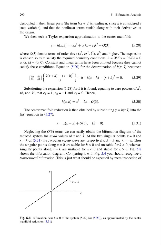
Neglecting the O(3) terms we can easily obtain the bifurcation diagram of the
reduced system for small values of x and k. At the two singular points x = 0 and
x = k of (5.31) the Jacobian eigenvalues are, respectively, k = k and k = −k. Thus
the singular points along x = 0 are stable for k < 0 and unstable for k > 0, whereas
singular points along x = k are unstable for k < 0 and stable for k > 0. Fig. 5.8
shows the bifurcation diagram. Comparing it with Fig. 5.4 you should recognize a
transcritical bifurcation. This is just what should be expected by mere inspection of
Fig. 5.8 Bifurcation near k = 0 of the system (5.22) (or (5.23)), as approximated by the center
manifold reduction (5.31)
290
5 Bifurcation Analysis
state variable), and that the nonlinear terms vanish along with their derivatives at
the origin.
We then seek a Taylor expansion approximation to the center manifold:
y ¼ hðx; kÞ ¼ c 1 x
2
þ c 2 kx þ c 3 k
2
þ Oð3Þ;
ð5:28Þ
where O(3) denote terms of order three (x
3 , kx
2 , k
2 x, k
3 ) and higher. The expansion
is chosen so as to satisfy the required boundary conditions, h = ∂h/∂x = ∂h/∂k = 0
at (x, k) = (0, 0). Constant and linear terms have been omitted because they cannot
satisfy these conditions. Equation (5.20) for the determination of h(x, k) becomes:
@h
@x
@h
@k
Â
à kðx þ hÞ À ðx þ hÞ
2
0
&
'
þ h þ kðx þ hÞ À ðx þ hÞ
2 ¼ 0:
ð5:29Þ
Substituting the expansion (5.28) for h it is found, equating to zero powers of x
2 ,
xk, and k
2 , that c 1 = 1, c 2 = −1 and c 3 = 0. Hence,
hðx; kÞ ¼ x
2
À kx þ Oð3Þ:
ð5:30Þ
The center manifold reduction is then obtained by substituting y = h(x,k) into the
first equation in (5.27):
_
x ¼ x k À x
ð
ÞþOð3Þ; ð _
k ¼ 0Þ:
ð5:31Þ
Neglecting the O(3) terms we can easily obtain the bifurcation diagram of the
reduced system for small values of x and k. At the two singular points x = 0 and
x = k of (5.31) the Jacobian eigenvalues are, respectively, k = k and k = −k. Thus
the singular points along x = 0 are stable for k < 0 and unstable for k > 0, whereas
singular points along x = k are unstable for k < 0 and stable for k > 0. Fig. 5.8
shows the bifurcation diagram. Comparing it with Fig. 5.4 you should recognize a
transcritical bifurcation. This is just what should be expected by mere inspection of
Fig. 5.8 Bifurcation near k = 0 of the system (5.22) (or (5.23)), as approximated by the center
manifold reduction (5.31)
290
5 Bifurcation Analysis