

5.3.2 The Saddle-node Bifurcation
For describing the saddle-node bifurcation we consider the generic system
_
x ¼ l À x
2
:
ð5:7Þ
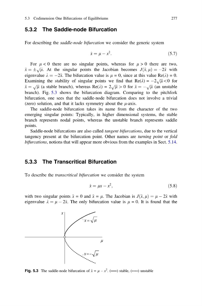
For l < 0 there are no singular points, whereas for l > 0 there are two,
~ x ¼ Æ
ffiffiffi
l
p . At the singular points the Jacobian becomes Jð~ x; lÞ ¼ À2~ x with
eigenvalue k ¼ À2~ x. The bifurcation value is l = 0, since at this value Re(k) = 0.
Examining the stability of singular points we find that Re(k) = À2
ffiffiffi
l
p \0 for
~ x ¼
ffiffiffi
l
p (a stable branch), whereas Re(k) = 2
ffiffiffi
l
p [ 0 for ~ x ¼ À
ffiffiffi
l
p (an unstable
branch). Fig. 5.3 shows the bifurcation diagram. Comparing to the pitchfork
bifurcation, one sees that the saddle-node bifurcation does not involve a trivial
(zero) solution, and that it lacks symmetry about the l-axis.
The saddle-node bifurcation takes its name from the character of the two
emerging singular points: Typically, in higher dimensional systems, the stable
branch represents nodal points, whereas the unstable branch represents saddle
points.
Saddle-node bifurcations are also called tangent bifurcations, due to the vertical
tangency present at the bifurcation point. Other names are turning point or fold
bifurcations, notions that will appear more obvious from the examples in Sect. 5.14.
5.3.3 The Transcritical Bifurcation
To describe the transcritical bifurcation we consider the system
_
x ¼ lx À x
2
;
ð5:8Þ
with two singular points ~ x = 0 and ~ x = l. The Jacobian is Jð~ x; lÞ ¼ l À 2~ x with
eigenvalue k ¼ l À 2~ x. The only bifurcation value is l = 0. It is found that the
Fig. 5.3 The saddle-node bifurcation of ~ x = l – x
2
. (
) stable, (
) unstable
5.3 Codimension One Bifurcations of Equilibriums
277
For describing the saddle-node bifurcation we consider the generic system
_
x ¼ l À x
2
:
ð5:7Þ
For l < 0 there are no singular points, whereas for l > 0 there are two,
~ x ¼ Æ
ffiffiffi
l
p . At the singular points the Jacobian becomes Jð~ x; lÞ ¼ À2~ x with
eigenvalue k ¼ À2~ x. The bifurcation value is l = 0, since at this value Re(k) = 0.
Examining the stability of singular points we find that Re(k) = À2
ffiffiffi
l
p \0 for
~ x ¼
ffiffiffi
l
p (a stable branch), whereas Re(k) = 2
ffiffiffi
l
p [ 0 for ~ x ¼ À
ffiffiffi
l
p (an unstable
branch). Fig. 5.3 shows the bifurcation diagram. Comparing to the pitchfork
bifurcation, one sees that the saddle-node bifurcation does not involve a trivial
(zero) solution, and that it lacks symmetry about the l-axis.
The saddle-node bifurcation takes its name from the character of the two
emerging singular points: Typically, in higher dimensional systems, the stable
branch represents nodal points, whereas the unstable branch represents saddle
points.
Saddle-node bifurcations are also called tangent bifurcations, due to the vertical
tangency present at the bifurcation point. Other names are turning point or fold
bifurcations, notions that will appear more obvious from the examples in Sect. 5.14.
5.3.3 The Transcritical Bifurcation
To describe the transcritical bifurcation we consider the system
_
x ¼ lx À x
2
;
ð5:8Þ
with two singular points ~ x = 0 and ~ x = l. The Jacobian is Jð~ x; lÞ ¼ l À 2~ x with
eigenvalue k ¼ l À 2~ x. The only bifurcation value is l = 0. It is found that the
Fig. 5.3 The saddle-node bifurcation of ~ x = l – x
2
. (
) stable, (
) unstable
5.3 Codimension One Bifurcations of Equilibriums
277