

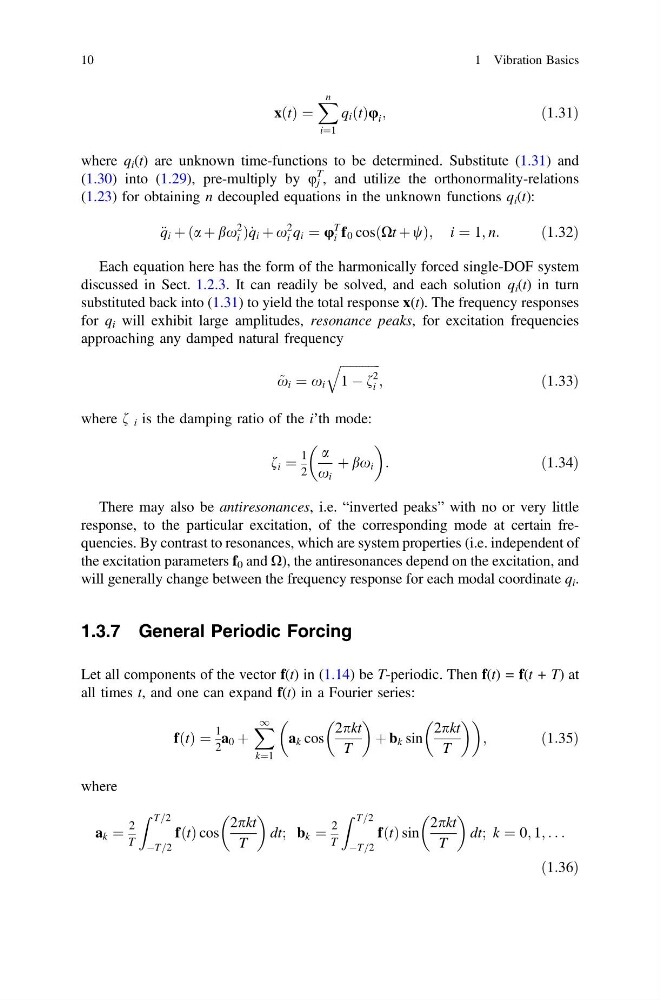
xðtÞ ¼
X n
i¼1
q i ðtÞu i ;
ð1:31Þ
where q i (t) are unknown time-functions to be determined. Substitute (1.31) and
(1.30) into (1.29), pre-multiply by φ j
T , and utilize the orthonormality-relations
(1.23) for obtaining n decoupled equations in the unknown functions q i (t):
€ q i þ ða þ bx
2
i Þ _
q i þ x
2
i q i ¼ u
T
i f 0 cosðXt þ wÞ; i ¼ 1; n:
ð1:32Þ
Each equation here has the form of the harmonically forced single-DOF system
discussed in Sect. 1.2.3. It can readily be solved, and each solution q i (t) in turn
substituted back into (1.31) to yield the total response x(t). The frequency responses
for q i will exhibit large amplitudes, resonance peaks, for excitation frequencies
approaching any damped natural frequency
~
x i ¼ x i
ffiffiffiffiffiffiffiffiffiffiffiffi ffi
1 À f
2
i
q
;
ð1:33Þ
where f i is the damping ratio of the i’th mode:
f i ¼
1
2
a
x i
þ bx i
:
ð1:34Þ
There may also be antiresonances, i.e. “inverted peaks” with no or very little
response, to the particular excitation, of the corresponding mode at certain frequencies. By contrast to resonances, which are system properties (i.e. independent of
the excitation parameters f 0 and X), the antiresonances depend on the excitation, and
will generally change between the frequency response for each modal coordinate q i .
1.3.7 General Periodic Forcing
Let all components of the vector f(t) in (1.14) be T-periodic. Then f(t) = f(t + T) at
all times t, and one can expand f(t) in a Fourier series:
fðtÞ ¼
1
2
a 0 þ
X 1
k¼1
a k cos
2pkt
T
þ b k sin
2pkt
T
;
ð1:35Þ
where
a k ¼
2
T
Z T=2
ÀT=2
fðtÞ cos
2pkt
T
dt; b k ¼
2
T
Z T=2
ÀT=2
fðtÞ sin
2pkt
T
dt; k ¼ 0; 1; . . .
ð1:36Þ
10
1 Vibration Basics
X n
i¼1
q i ðtÞu i ;
ð1:31Þ
where q i (t) are unknown time-functions to be determined. Substitute (1.31) and
(1.30) into (1.29), pre-multiply by φ j
T , and utilize the orthonormality-relations
(1.23) for obtaining n decoupled equations in the unknown functions q i (t):
€ q i þ ða þ bx
2
i Þ _
q i þ x
2
i q i ¼ u
T
i f 0 cosðXt þ wÞ; i ¼ 1; n:
ð1:32Þ
Each equation here has the form of the harmonically forced single-DOF system
discussed in Sect. 1.2.3. It can readily be solved, and each solution q i (t) in turn
substituted back into (1.31) to yield the total response x(t). The frequency responses
for q i will exhibit large amplitudes, resonance peaks, for excitation frequencies
approaching any damped natural frequency
~
x i ¼ x i
ffiffiffiffiffiffiffiffiffiffiffiffi ffi
1 À f
2
i
q
;
ð1:33Þ
where f i is the damping ratio of the i’th mode:
f i ¼
1
2
a
x i
þ bx i
:
ð1:34Þ
There may also be antiresonances, i.e. “inverted peaks” with no or very little
response, to the particular excitation, of the corresponding mode at certain frequencies. By contrast to resonances, which are system properties (i.e. independent of
the excitation parameters f 0 and X), the antiresonances depend on the excitation, and
will generally change between the frequency response for each modal coordinate q i .
1.3.7 General Periodic Forcing
Let all components of the vector f(t) in (1.14) be T-periodic. Then f(t) = f(t + T) at
all times t, and one can expand f(t) in a Fourier series:
fðtÞ ¼
1
2
a 0 þ
X 1
k¼1
a k cos
2pkt
T
þ b k sin
2pkt
T
;
ð1:35Þ
where
a k ¼
2
T
Z T=2
ÀT=2
fðtÞ cos
2pkt
T
dt; b k ¼
2
T
Z T=2
ÀT=2
fðtÞ sin
2pkt
T
dt; k ¼ 0; 1; . . .
ð1:36Þ
10
1 Vibration Basics