

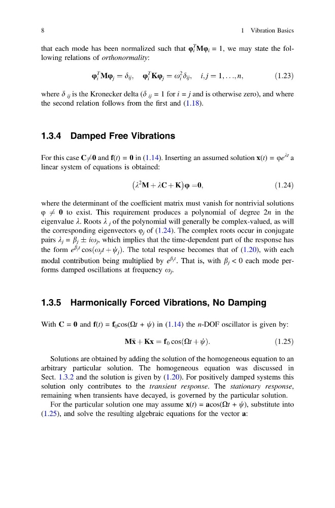
that each mode has been normalized such that φ i
T
Mφ i = 1, we may state the following relations of orthonormality:
u
T
i Mu j ¼ d ij ; u
T
i Ku j ¼ x
2
i d ij ; i; j ¼ 1; . . .; n;
ð1:23Þ
where d ij is the Kronecker delta (d ij = 1 for i = j and is otherwise zero), and where
the second relation follows from the first and (1.18).
1.3.4 Damped Free Vibrations
For this case C6 ¼0 and f(t) = 0 in (1.14). Inserting an assumed solution x(t) = φe
kt a
linear system of equations is obtained:
k
2
M þ kC þ K
À
Á u ¼0;
ð1:24Þ
where the determinant of the coefficient matrix must vanish for nontrivial solutions
φ 6 ¼ 0 to exist. This requirement produces a polynomial of degree 2n in the
eigenvalue k. Roots k j of the polynomial will generally be complex-valued, as will
the corresponding eigenvectors φ j of (1.24). The complex roots occur in conjugate
pairs k j = b j ± ix j , which implies that the time-dependent part of the response has
the form e
b j t cosðx j t þ w j Þ. The total response becomes that of (1.20), with each
modal contribution being multiplied by e
b j t . That is, with b j < 0 each mode performs damped oscillations at frequency x j .
1.3.5 Harmonically Forced Vibrations, No Damping
With C = 0 and f(t) = f 0 cos(Xt + w) in (1.14) the n-DOF oscillator is given by:
M€ x þ Kx ¼ f 0 cosðXt þ wÞ:
ð1:25Þ
Solutions are obtained by adding the solution of the homogeneous equation to an
arbitrary particular solution. The homogeneous equation was discussed in
Sect. 1.3.2 and the solution is given by (1.20). For positively damped systems this
solution only contributes to the transient response. The stationary response,
remaining when transients have decayed, is governed by the particular solution.
For the particular solution one may assume x(t) = acos(Xt + w), substitute into
(1.25), and solve the resulting algebraic equations for the vector a:
8
1 Vibration Basics
T
Mφ i = 1, we may state the following relations of orthonormality:
u
T
i Mu j ¼ d ij ; u
T
i Ku j ¼ x
2
i d ij ; i; j ¼ 1; . . .; n;
ð1:23Þ
where d ij is the Kronecker delta (d ij = 1 for i = j and is otherwise zero), and where
the second relation follows from the first and (1.18).
1.3.4 Damped Free Vibrations
For this case C6 ¼0 and f(t) = 0 in (1.14). Inserting an assumed solution x(t) = φe
kt a
linear system of equations is obtained:
k
2
M þ kC þ K
À
Á u ¼0;
ð1:24Þ
where the determinant of the coefficient matrix must vanish for nontrivial solutions
φ 6 ¼ 0 to exist. This requirement produces a polynomial of degree 2n in the
eigenvalue k. Roots k j of the polynomial will generally be complex-valued, as will
the corresponding eigenvectors φ j of (1.24). The complex roots occur in conjugate
pairs k j = b j ± ix j , which implies that the time-dependent part of the response has
the form e
b j t cosðx j t þ w j Þ. The total response becomes that of (1.20), with each
modal contribution being multiplied by e
b j t . That is, with b j < 0 each mode performs damped oscillations at frequency x j .
1.3.5 Harmonically Forced Vibrations, No Damping
With C = 0 and f(t) = f 0 cos(Xt + w) in (1.14) the n-DOF oscillator is given by:
M€ x þ Kx ¼ f 0 cosðXt þ wÞ:
ð1:25Þ
Solutions are obtained by adding the solution of the homogeneous equation to an
arbitrary particular solution. The homogeneous equation was discussed in
Sect. 1.3.2 and the solution is given by (1.20). For positively damped systems this
solution only contributes to the transient response. The stationary response,
remaining when transients have decayed, is governed by the particular solution.
For the particular solution one may assume x(t) = acos(Xt + w), substitute into
(1.25), and solve the resulting algebraic equations for the vector a:
8
1 Vibration Basics