

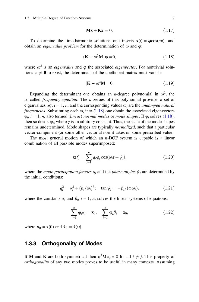
M€ x þ Kx ¼ 0:
ð1:17Þ
To determine the time-harmonic solutions one inserts x(t) = ucos(xt), and
obtain an eigenvalue problem for the determination of x and u:
ðK À x
2
MÞu ¼0;
ð1:18Þ
where x
2 is an eigenvalue and u the associated eigenvector. For nontrivial solutions φ 6 ¼ 0 to exist, the determinant of the coefficient matrix must vanish:
K À x
2
M
¼0:
ð1:19Þ
Expanding the determinant one obtains an n-degree polynomial in x
2 , the
so-called frequency-equation. The n zeroes of this polynomial provides a set of
eigenvalues x
2
i , i = 1, n, and the corresponding values x i are the undamped natural
frequencies. Substituting each x i into (1.18) one obtain the associated eigenvectors
φ i , i = 1, n, also termed (linear) normal modes or mode shapes. If φ i solves (1.18),
then so does c φ i , where c is an arbitrary constant. Thus, the scale of the mode shapes
remains undetermined. Mode shapes are typically normalized, such that a particular
vector-component (or some other vectorial norm) takes on some prescribed value.
The most general motion of which an n-DOF system is capable is a linear
combination of all possible modes superimposed:
xðtÞ ¼
X n
i¼1
q i u i cosðx i t þ w i Þ;
ð1:20Þ
where the mode participation factors q i and the phase angles w i are determined by
the initial conditions:
q
2
i ¼ a
2
i þ ðb i =x i Þ
2 ; tan w i ¼ Àb i =ða i x i Þ;
ð1:21Þ
where the constants a i and b i , i = 1, n, solves the linear systems of equations:
X n
i¼1
u i a i ¼ x 0 ;
X n
i¼1
u i b i ¼ _
x 0 ;
ð1:22Þ
where x 0 = x(0) and _
x 0 ¼ _
xð0Þ.
1.3.3 Orthogonality of Modes
If M and K are both symmetrical then φ i
T
Mφ j = 0 for all i 6 ¼ j. This property of
orthogonality of any two modes proves to be useful in many contexts. Assuming
1.3 Multiple Degree of Freedom Systems
7
ð1:17Þ
To determine the time-harmonic solutions one inserts x(t) = ucos(xt), and
obtain an eigenvalue problem for the determination of x and u:
ðK À x
2
MÞu ¼0;
ð1:18Þ
where x
2 is an eigenvalue and u the associated eigenvector. For nontrivial solutions φ 6 ¼ 0 to exist, the determinant of the coefficient matrix must vanish:
K À x
2
M
¼0:
ð1:19Þ
Expanding the determinant one obtains an n-degree polynomial in x
2 , the
so-called frequency-equation. The n zeroes of this polynomial provides a set of
eigenvalues x
2
i , i = 1, n, and the corresponding values x i are the undamped natural
frequencies. Substituting each x i into (1.18) one obtain the associated eigenvectors
φ i , i = 1, n, also termed (linear) normal modes or mode shapes. If φ i solves (1.18),
then so does c φ i , where c is an arbitrary constant. Thus, the scale of the mode shapes
remains undetermined. Mode shapes are typically normalized, such that a particular
vector-component (or some other vectorial norm) takes on some prescribed value.
The most general motion of which an n-DOF system is capable is a linear
combination of all possible modes superimposed:
xðtÞ ¼
X n
i¼1
q i u i cosðx i t þ w i Þ;
ð1:20Þ
where the mode participation factors q i and the phase angles w i are determined by
the initial conditions:
q
2
i ¼ a
2
i þ ðb i =x i Þ
2 ; tan w i ¼ Àb i =ða i x i Þ;
ð1:21Þ
where the constants a i and b i , i = 1, n, solves the linear systems of equations:
X n
i¼1
u i a i ¼ x 0 ;
X n
i¼1
u i b i ¼ _
x 0 ;
ð1:22Þ
where x 0 = x(0) and _
x 0 ¼ _
xð0Þ.
1.3.3 Orthogonality of Modes
If M and K are both symmetrical then φ i
T
Mφ j = 0 for all i 6 ¼ j. This property of
orthogonality of any two modes proves to be useful in many contexts. Assuming
1.3 Multiple Degree of Freedom Systems
7