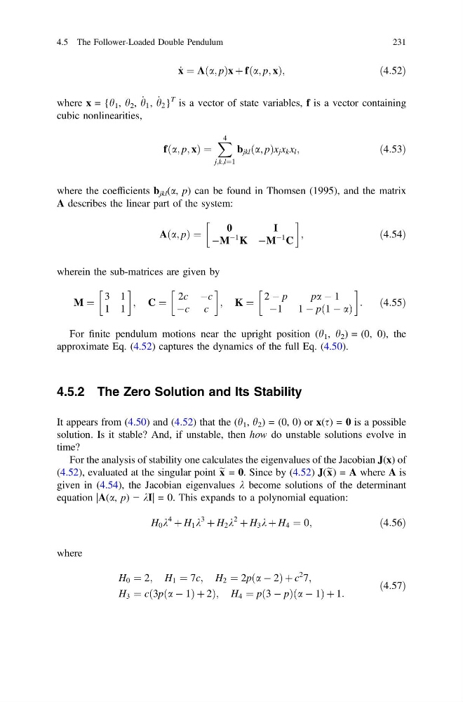
_
x ¼ Aða; pÞx þ fða; p; xÞ;
ð4:52Þ
where x = {h 1 , h 2 , _
h 1 , _
h 2 }
T is a vector of state variables, f is a vector containing
cubic nonlinearities,
fða; p; xÞ ¼
X 4
j;k;l¼1
b jkl ða; pÞx j x k x l ;
ð4:53Þ
where the coefficients b jkl (a, p) can be found in Thomsen (1995), and the matrix
A describes the linear part of the system:
Aða; pÞ ¼
0
I
ÀM
À1
K ÀM
À1
C
!
;
ð4:54Þ
wherein the sub-matrices are given by
M ¼
3 1
1 1
!
; C ¼
2c Àc
Àc c
!
; K ¼
2 À p
pa À 1
À1 1À pð1 À aÞ
!
:
ð4:55Þ
For finite pendulum motions near the upright position (h 1 , h 2 ) = (0, 0), the
approximate Eq. (4.52) captures the dynamics of the full Eq. (4.50).
4.5.2 The Zero Solution and Its Stability
It appears from (4.50) and (4.52) that the (h 1 , h 2 ) = (0, 0) or x(s) = 0 is a possible
solution. Is it stable? And, if unstable, then how do unstable solutions evolve in
time?
For the analysis of stability one calculates the eigenvalues of the Jacobian J(x) of
(4.52), evaluated at the singular point e x = 0. Since by (4.52) J(e x) = A where A is
given in (4.54), the Jacobian eigenvalues k become solutions of the determinant
equation |A(a, p) − kI| = 0. This expands to a polynomial equation:
H 0 k
4
þ H 1 k
3
þ H 2 k
2
þ H 3 k þ H 4 ¼ 0;
ð4:56Þ
where
H 0 ¼ 2; H 1 ¼ 7c; H 2 ¼ 2pða À 2Þ þ c
2 7;
H 3 ¼ c 3pða À 1Þ þ 2
ð
Þ ; H 4 ¼ pð3 À pÞða À 1Þ þ 1:
ð4:57Þ
4.5 The Follower-Loaded Double Pendulum
231